Performance Analysis of MPC in the Control of a Simple
Motorized Nonlinear Model of a Robotic Leg
Abdur Raquib Ridwan
Lecturer Islamic University of Technology, EEE Department
Md. Ibnea Sina Bony
Islamic University of Technology, EEE Department
Ishtiza Ibne Azad
Lecturer Islamic University of Technology, EEE Department
ABSTRACT
This paper presents a simple design and analysis of a robotic leg using MPC as a single degree of freedom motion controller. Performance of the Model Predictive Controller is compared with a generic adaptive PID controller. The rotational motion of a simple nonlinear model of a robotic leg is operated by a DC motor [1][2]. A desired rotation of the leg from 90 to 0 degree is taken as the controlling scenario for analyzing the performance of the Model Predictive Controller. This paper also presents the use of Matlab software for the purpose of a simple control system design [3][4]. Although a simple model is taken the concern of a desired angular rotation is solved by the use of MPC as the controller [6][7].
General Terms
NonlinearControl, Model Predictive Control, Simulink approach of Robotic Leg control.
Keywords
DC motor Control, PID Controller, Model Predictive Controller.
1.
INTRODUCTION
Modeling of a simple motion control system is the underlying foundation from which the development of a realistic complex autonomous control system is possible. In the field of automation engineering it is quintessential to be able to understand and evaluate the use of a specific controller. In this paper we have taken a DC motor operated Robotic leg as the simple nonlinear model for analysis [1][2]. The one degree of freedom rotation of this simple system is then controlled by a Model Predictive Controller. To evaluate its performance an adaptive PID controller is also used. The entire model is designed in the Matlab Simulink environment [4]. Finally a linearized state space model is obtained which finally gave us an insight about the stability of the system. Moreover, a classical approach was taken to understand the controllability of the simple system in this paper. A step trajectory of angles ranging from 0 to 90 degree corresponding to specific range of voltage which in this case was considered to be 0V to 10V was to be traced by our system. The performance and quality of response was judged on the basis of settling time, overshoot and steady state error obtained from the step responses at various tracking angles of the simple system presented in this paper.
In section 2 we took a simple nonlinear dynamic model of the robotic leg and integrated it with the linear model of a DC
section. Section 3 deals with the use of both MPC and PID controller on our system. Both the Simulink models along with optimum control parameters are given here. In Section 4 the simulation results generated from the Simulink environment of Matlab is shown and performance was compared based on the simulation results.A far better response was obtained when the robotic leg was controlled by MPC [6][8]. With section 5 we conclude the paper with references in section 6.
2.
Nonlinear Modeling of Robotic Human
Leg
2.1 Equivalent Model of Leg:
A robotic leg can be modeled taking into account a simplistic model of a human leg that relates the output angular rotation about the hip joint to the input torque generated by the leg muscle [2]. A simplified model for the robotic leg assumes an applied torque Tm supplied by the DC motor, viscous
[image:1.595.358.497.489.604.2]damping, D, at the hip joint, and inertia J, around the hip joint. Finally the component of the weight of the leg, Mg, where M is the mass of the leg and g is the acceleration due to gravity creates a nonlinear torque. Assuming the robotic leg to be of uniformdensity, the weight can be applied at L/2, where L is the length of the leg. A pictorial representation of the cylindrical model of a robotic human leg is shown below.
Figure 1: Cylindrical model of a Robotic Human leg
Summing the torques, the dynamic model of the robotic human leg can be obtained which is as follows:
( )
(2.1)2.2
Design method of DC motor operated
robotic Leg:
A DC motor with armature control and a fixed field is considered. The electrical model of such a DC motor is illustrated in Figure 2[10]. The armature voltage, ea(t) is the
voltage provided by an amplifier to control the motor. The motor has a resistance Ra, inductance La and back electromotive force constant, Kb. The back emf voltage, Vb (t)
is induced by the rotation of the armature windings in the fixed magnetic field. The counter emf is proportional to the speed of the motor with field strength fixed. The governing equations are as
follows:-( )
(2.2.1)
Taking the Laplace transform of equation 2.2.1 gives
[image:2.595.58.277.249.416.2]( )
(2.2.2)
Figure 2: DC motor (a) circuit diagram (b) Block diagram
The circuit equation for the electrical section of the motor can be written as
( )
( )
( )
( )
(2.2.3)The equation can also be written as:
( )
( ) ( ) (2.2.4)The torque developed by the motor is proportional to the armature current and the equation is as follows
( )
( )
(2.2,5) [image:2.595.358.498.590.718.2]Using the torque equation and the current equation a Simulink model of the DC motor operated robotic arm can be obtained [3][4]. The figure is shown below:
Figure 3: Simulink Model of the Nonlinear Robotic Human Leg by DC Motor
3.
Nonlinear Model Reference with PID
and MPC Based Controller
3.1
PID Controller Simulink Modeling:
To control the robotic leg such that the DC motor can rotate it from 0 degrees to 90 degrees, a PID controller is first of all installed so that it can give the accurate actuating signal for the desired response of the DC motor operated robotic leg model. The PID controller used for this purpose is an adaptive PID controller which also includes a filter block to obtain the most efficient response. The PID block uses the compensator formula [1][9] which is:
(3.1)
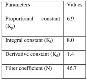
Where Kp is the proportional constant, Ki is the integral
constant, Kd is the derivative constant and N is known as the
filter coefficient.
The optimized values [3][4] used for the PID controller is tabulated as follows:
Table1: Optimized values for PID controller
Parameters Values
Proportional constant (Kp)
6.9
Integral constant (Ki) 8.0
Derivative constant (Kd) 1.4
The Simulink model of the PIDcontroller [9] is as follows:
Figure 4: A Simulink Model of PID Controller
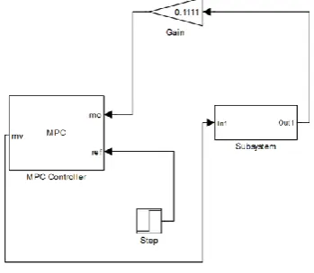
The Simulink model incorporating the PID controller is shown below:
Figure 5: Simulink Model of Robotic Human Leg with PID Controller with the robotic leg represented in the
form of a subsystem.
The system input is a voltage signal with a range from 0 to 10 V. This signal is used to provide the control voltage and current to the DC motor. The goal is to design a controller so that a voltage ranging from 0 to 10 volts corresponds linearly to an angular rotation of a robotic arm from 0 to 90 degree respectively. Since we want to move the robotic human leg to a proper angular position corresponding to the input, a positional servomechanism will be needed to convert the angular position information into corresponding voltage and negatively feedback the signal back into the system so that it can be compared with the input voltage signal and fed to the input of the controller. The feedback signal in voltage is Ef=
θL×Kpwhere Kp is the proportional constant and is equal to
the ratio of the input to the desired position output. In our case 10V should correspond to 90 degree. Hence Kpwhich also known as the Load angle Velocity feedback will be equal to 10/90 = 0.1111.
3.2
MPC
Controller
Based
Simulink
Modeling:
The model predictive controller (MPC) is designed depending upon the past inputs and outputs, model predicts the future output [8]. It is compared with reference value and the subtracted result or future error is sent to theoptimizer.With
reaches close to the desired reference value [6][7]. A basic structure of MPC [8] in block diagrams is shown below:
Model
Optimizer
Past inputs and outputs
Predicted output
Future inputs
Future errors
Reference trajectory
+
-Cost function -Costraints
[image:3.595.330.537.98.326.2]Figure 6: Basic Structure of MPC
[image:3.595.62.272.290.408.2]The model predictive controller is designed by tuning different parameters for obtaining the best response. The parameters finally chosen for controlling our system are shown in the tabular format as follows:
Table 2: Parameters for MPC
Parameters Values
Control Interval 0.1
Prediction Horizon 10
Control Horizon 2
[image:3.595.351.505.425.531.2] [image:3.595.320.495.576.728.2]4.
Comparative Analysis of Simulation
Result:
A comparative analysis of the performance of the robotic leg by both MPC and PID controller is obtained by undergoing simulations in Matlab [3][5]. Signal values ranging from 10V to 4V is chosen and the desired output for such actuating signals should be from 90 to 30 degree respectively.
The response of the system using the PID controller for an input of 10 volts is shown below:
Figure 8
The settling time for the system is 0.04 seconds but the overshoot is around 8%. Such a overshoot is not desirable for the system.
The response of the system using the MPC controller for an input of 10 volts is shown below:
Figure 9
While using the MPC controller the settling time has reduced down to 0.037 seconds and overshoot has been totally eliminated.
The response of the system using the PID controller for a input signal of 4 volts is shown below:
Figure 10
The output was way beyond the desired angle of 30 degrees. A steady state error of 5% was obtained. The response was very poor.
Carrying out the same operation using MPC controller we got a far better response as shown below:
Figure 11
In the case we obtained a settling time of 0.025 seconds and no overshoot at all.
This simple nonlinear model [5] was linearized using Taylor series method and the state space model used by the MPC controller was
[ ̇̇] [
] [ ] [ ] (4.1)
(4.2)
Where =θ.
The corresponding transfer function of the linear model is described as follows:
( ) ( )
The eigenvalues of the system matrix were -1.3285 + 3.1568i & -1.3285 - 3.1568i showing that the system is stable because the real parts of the eigenvalues are negative.
0 0.05 0.1 0.15 0.2 0.25 0.3 0.35 0.4 0.45 0.5 50
55 60 65 70 75 80 85 90 95 100
Time(Seconds)
A
n
g
l
e
(
d
e
g
r
e
e
s
5.
Conclusion
In this paper we tried to implement a simple model of a robotic leg with a DC motor rotation in response to a specified Voltage[2]. Our motto was to show the superlative performance of Model predictive controller over PID controller in controlling small systems. This simulation results prove our concept and this allow us to use MPC for more complex systems.
This paper also presents the process of implementing simple control system design using the Simulink environment of the Matlab Software [3][4].
Our future work will be on the application of MPC in more complex systems such as multi direction rotation of human leg and to stabilize the system for different inputs.
6. References
[1]
“
Modeling, control and experimental characterization of microbiorobots” by Mahmut Selman Sakar, Edward B Steager, Dal Hyung Kim, A Agung Julius, MinJun Kim, Vijay Kumar and George J Pappas. The International Journal of Robotics Research 2011 30: 647–658. [2] Chun HtooAung, KhinThandarLwin, and Yin MonMyint "Modeling Motion Control System for Motorized Robot Arm using MATLAB", World Academy of Science, Engineering and Technology 42 2008.
[3] Mathworks, 2011.[4] MPC toolbox in Simulink, 2011. [4] MPC toolbox in Simulink, 2011.
[5] D.E. Seborg, T.E. Edgar, D.A. Mellichamp, “Process Dynamics and Control”, second ed., John Wiley, Hoboken, NJ, 2004.
[6] Rawlings, J. B., Meadows, E. S., &Muske, K. R., “Nonlinear model predictive control: A tutorial and survey”. ADCHEM'94 Proceedings, Kyoto, Japan (pp. 185,197), 1994.
[7] Qin S.J. and BadgwellT.A,“An overview of nonlinear model predictive control applications”, In F. Allg¨ower and A. Zheng, editors, “Nonlinear Predictive Control”,
pages 369–
393. Birkh¨auser, 2000.
[8] Eduardo F, Camacho and Carlos Bordons: “Model Predictive Control Advanced Textbooks in Control and Signal Processing”, Springer Publication, 1998