Active Contour without Edges vs GVF Active Contour for Accurate Pupil Segmentation

Active Contour without Edges Vs GVF Active Contour

for Accurate Pupil Segmentation

Walid AYDI

PhD student, University of sfax Laboratory of Electronics and

Information Technologies Sfax, Tunisia

Nouri MASMOUDI

Professor, University of sfax Laboratory of Electronics and

Information Technologies Sfax, Tunisia

Lotfi KAMOUN

Professor, University of sfax Laboratory of Electronics and

Information Technologies Sfax, Tunisia

ABSTRACT

Iris localization is a critical step for an iris recognition system because it directly affects the recognition rates. Consequently, in order to have reasonably accurate measures, we should estimate as many iris boundaries as possible which are defined by papillary and ciliary regions. Due to the contraction which is an intrinsic propriety of the pupil and the variations in the shooting angle, the pupil will not be a regular circle. So an active contour is suitable to accurately locate the iris boundaries. In this paper we focused on iris/pupil boundary and we proposed a new algorithm based on an active contour without edges applied in gray level image. First, we develop a new method to locate and fill the corneal reflection which is used not only to remove the highlight points that appear inside the pupil but also as an initial contour generator for the snake. Second, we propose to use the active contour without edges for precise pupil segmentation. This kind of snake can detect objects whose boundaries are not necessarily defined by gradient. Our algorithm seems to be robust to occlusion, specular reflection, variation in illumination and improves its efficiency in precision and time computation compared with AIPF and Gvf active contour. Another advantage is that the initial curve can be anywhere in the image and the contour will be automatically detected.

The proposed algorithm is 2.36 faster than GVF snake-based method for accurate pupil contour detection and integro-differential method with accuracy up to 99.62% using CASIA iris database V3.0 and up to 100% with CASIA iris database V1.0.

Keywords

Iris, pupil, snake, specular reflection, active contour without edges.

1. INTRODUCTION

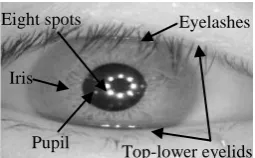
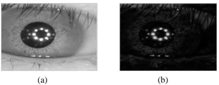
Security has become a major aspect, mainly in areas that require high security levels. For many users, the safest way to protect themselves is to use biometrics. The iris is the ‘‘colored ring of tissue around the pupil through which light enters the interior of the eye” [26]. It has a complex pattern which contains many distinctive features like furrows, arching ligaments, ridges, crypts, rings, corona, freckles, and the collarette [3]. Figure 1 shows an example image from Casia V3.0.

The iris recognition system is one of the most important and reliable techniques [1, 2] aging invariant, compared with other biometric systems. Such an iris recognition system has four main stages: segmentation, normalization, encoding and matching. The first iris recognition system was proposed by

Daugman who assumed iris boundaries by two circles using integro-differential operator [3, 25]. After that many other algorithms, based on the edge maps [4], have appeared. Wildes and Masek [5, 6] used edge detection followed by the Hough transforms to detect the iris boundaries and both are circle models. Another proposition assumes the iris and the pupil as an elliptic form [7, 8]. However, these methods are not so good in particular for noisy, blurred and off-angle irises. As a consequence a papillary or ciliary boundary is not perfectly circular and therefore can lead to inaccuracy if fitted with simple shape assumptions (circle, ellipse). To overcome the disadvantages related to the non regularity of the pupil and iris shapes, many algorithms have been proposed. Daugman suggested a novel algorithm based on discrete Fourier series expansions of the contour data [9]. Zhaofeng HE suggested a novel method based on Hooke’s law, called Pulling & Pushing [10] and Kien proposed to use fusing, shrinking and expanding active contour models [11], Ann Jarjes proposed to use the AIPF and Gvf active contour for a more precise detection.

In this paper we presented a new method for the detection of the precise pupil contour which is based on the active contour without edges. We defined a modified corneal reflection removal method [24] not only used to remove the corneal reflection inside the pupil but also to give an initial contour for the snake. Using the mask generated by the first process and taking into account that the pupil region is darker than the iris region, we proposed to use the active contour without edges which is a very robust technique used to separate two objects with a difference between the foreground and background means.

[image:1.595.367.495.661.740.2]

The remaining of this paper is organized as follows: In section II we gave an explanation of two iris segmentation methods using integro differential operator [3] and GVF active contour [12]. Section three dealt with the proposed algorithm based on an active contour without edges. In the fourth section, however, we described Chan Vese algorithm used to precisely segment the pupil region, and then we assessed our algorithm and presented our experimental results. Finally, conclusions were drawn in section 5.

Fig 1: Example of iris image from CASIA V3.0. Iris

Eyelashes Eight spots

Pupil

International Journal of Computer Applications (0975 – 8887) Volume 54– No.4, September 2012

2. BACKGROUND

2.1

Daugman Approach:

Daugman’s approach [3] is based on an integro-differenrential operator to localize the iris regions using equation (1):

 

 

*

 

,

₂

 

1

max

0 0 0

0, _{, ,}

,

_





y x r y

x

r

_r

ds

y

x

I

r

r

G

_

_

The integro differential operator looks for the maximum value of the blurred partial derivatives over the image domain,

according to a circular arc

ds

of radius r and center



x

0

,

y

0



.

 

r

G

_ is a smoothing function used to blur the iris texture. Depending on the nature of the desired edges, the value of sigma can take two distinct values, great and low, to detect the pupil. Soon, the new methods assume the pupil region with an irregular shape [9, 12, 11]. It seems more suitable to replace this assumption by other methods that can model the pupil boundaries whatever their shapes are.

2.2

GVF Active Contour Based Method for

accurate pupil contour detection

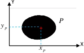
In [12], Ann JARJES proposes a new method for pupil boundary localization based on GVF active contour and AIPF to refine the pupil boundary. This method is made up of four steps: image denoising and enhancement, pupil center estimation, circular pupil localization and precise pupil contour detection. The flowchart in Figure 2 describes all the modules of this algorithm. The first step named image denoising and enhancement gives a cleaner image without reflection spots. We could remind here that this technique was tested in our paper [24]. In the second step it follows a fine estimation of pupil radius

R

_pand center which coincides with its center of mass as shown in Figure 3. Pupil center coordinates



x

_p

,

y

_p



and the radius are determined using the equations (2) and (3):

   

 

2

1

,

1

,

,





 





P j i I p p

P j i I p

p

_n

i

y

_n

j

x

 

 ,

,

,



 

3

p p P

j i I p

S

R

j

i

I

S









Where,

n

_p is the number of pixels belonging to

P

and

S

_p

[image:2.595.302.569.78.508.2]

the corresponding area which equals the sum of pixels.

Fig 2: Flowchart of the GVF snake based method for accurate pupil contour detection

[image:2.595.366.507.622.711.2]

After the second step, and in order to refine the pupil boundary Ann JARJES uses the AIPF, the least square method and GVF active contour.

Fig 3: Pupil center approximation Image denoising and enhancement

Pupilcenterestimation

Original Image

Image Complement

Filling Holes

ImageComplement

ImageSmoothing

ImageThresholding

EyelashesElimination MiddleSubImage

ApproximationofPupil Center

Pupilcirclelocalization

Precisepupilcontour detection

P

X

+

p

y

p

2.2.1.

Angular Integral Projection

Function

(AIPF)

The first methods used to perform image projection are:

IPFv

(vertical integral projection function) and

IPFh

(horizontal integral projection function) that can be reformulated by the equations (4) and (5):

 

2





 

4 1

, dx

x xI x y x

h

IPF  _

 

2





 

5

1

,

dy

y

y

I

x

y

y

v

IPF



_

For the discrete implementation, it’s more efficient to replace

integrals with sums and

 

x

,

y

with

 

i

,

j

. With these manipulations we can derive an efficient discrete operator in the row and column direction defined by equations (6) and (7).

 

,

 

 

6

,

,





n

m

j

i

I

i

j

i

IPFh

 

,

 

 

7

,

,





n

m

i

j

I

i

j

j

IPFv

Where

I

 

i

,

j

is the intensity of a pixel at location

 

i

,

j

. These two operators (

IPFv

and

IPFh

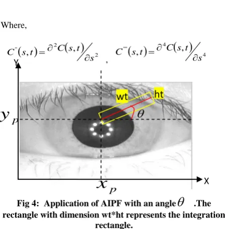
) have shown their inadequacies because they are limited to vertical and horizontal directions. That’s why a new method has appeared to perform an integral projection along angular directions [12] defined by AIPF in equation (8). The angular integral projection function performs line integration within a specific rectangle that extends from the pupil center and has angle with x axis as shown in Figure 4.



_{  }

2

 

8

2 sin sin ₂

, 2 cos cos 1 1 , , dh ht

ht _{r h}

p y h r p x I ht ht r AIPF _  _                                     

Where,

r





0

,

w

_t



is defined as the distance from the pupil center and







0

:

2





the integration angle. After the detection of a set of pupil boundary points using the AIPF technique, Ann JARJES used the least mean square to fit the curve that best describes these sets of points. After that it follows a GVF active contour, in order to refine the pupil boundary better. The parametric representation of GVF active

contour is

C

     

s





x

s

,

y

s



. Where s is the control parameter situated between [0, 1]. The total energy (as a sum

of an internal and external energy

E

_ext) of the snake [15] is defined by equation (9):

 

 



 

  

9

2

1

' 2 " 2

1 0

ds

s

C

E

s

C

s

C

E

























ext

Where,



and



are the elasticity and stiffness coefficients respectively. The corresponding dynamic snake is made through treating C as function of time t. Then the partial derivative of C is given by equation (10):

 

,

"

 

,

""

 

,

_ext

 

10

t

s

t

C

s

t

C

s

t

E

C













Where,

 

 

2 2 " , , s t s C t s

C  _

,

 

 

4 4 " " , , s t s C t s

[image:3.595.315.539.190.418.2]

C  _

Fig 4: Application of AIPF with an angle



.The rectangle with dimension wt*ht represents the integration

rectangle.

Although this method uses Gvf active contour to best refine the pupil region, there are some problems. First, in the image deionizing and enhancement stage this method is not good enough especially for the smaller pupil (where the several eight spots are almost equal to the pupil) (Figure 5-a), a bright pupil (Figure 5-b) and with a deflected reflection spots inside the iris region (Figure 5-c). After image deionizing, the pupil with a smaller region, will have almost the same gray level values as iris region which makes the image binarization using gray level histogram more difficult (Figure 5-d). Moreover, the eight spots inside the bright pupil (Figure 5-e) are not totally removed. To overcome these problems, we propose a new corneal reflection removal method based on the Top-hat as explained in section 3.Second, it is well known that the snake initialization accuracy influences significantly the segmentation and especially the time computing process. In GVF active contour method the accuracy of the initial contour and the execution time are closely linked to the number of initial contour points. If we want to have a precise initial contour we should have a lot of initial points; thus more computing time. In order to overcome the problem related to active contour initialization and the waste of time computation we can use the edge map of the pupil to generate the first contour based on the level set method and Signed Distance Function(SDF). The well known active contour without edges is then used to precisely segment the iris region using the first contour generated from the intersection between SDF and the level set zero.

(a) (b) (c)

[image:4.595.304.570.70.466.2]

(d) (e) (f)

Fig 5: Results of image deinoising and enhancement. (a-c) Original image from Casia-V3.0. (d) Image processed with

small pupil. (e) Image processed with highlight pupil. (f) Image processed with deflected reflection spots inside

the iris region

3. PROPOSED METHOD

An iris and a pupil are two separate objects because of the sharp contrast between them [16]. The pupil region appears darker than that of the iris. Using this propriety we can assume the pupil as a foreground and the iris as a background statistically different.

In order to separate the pupil from the iris region we use an active contour without edges. This technique deforms an initial curve so that it separates the foreground from the background based on the means of the two regions [17]. The technique is very robust to initialization and gives good results because of the high difference between the foreground (pupil) and background (iris) means.

Our used method to detect the pupil region consists of two main stages. The first is a primary reduction of corneal reflections and initial contour generator. The second stage is the pupil boundary localization using an active contour without edges to accurately segment the pupil region. In order to avoid the divergence of an active contour, we should take into consideration the typical sources of noise including the corneal reflection and eyelashes.

3.1

Corneal Reflection removal

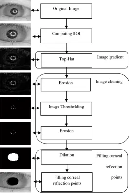
[image:4.595.49.292.76.255.2]

Corneal reflection removal is a crucial step. It is used not only to denoise the pupil but also to estimate its position. Earlier we have developed a method for a corneal reflection removal method [24]. Here we introduce some modifications in order to focus on the eight spots inside the pupil. Thus, the four major stages included in this approach are as follows: computing ROI (Region Of Interest), Image gradient, Image cleaning and Filling corneal reflection points, as illustrated by the flowchart given in Figure 6.

Fig 6: Flowchart of corneal reflection removal method.

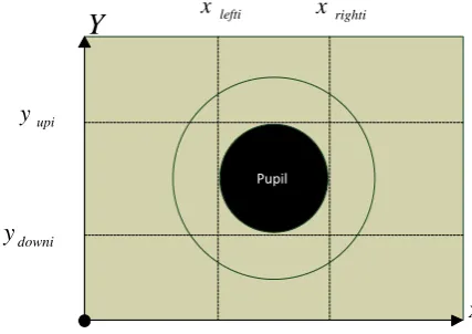
3.1.1.

Computing ROI

Through analyzing the full CASIA iris image database V3.0

we determined the boundaries limits



x

upi

,

x

downi

,

y

lefti

,

y

righti



of each pupil in CASIA iris

database V3.0, as shown in Figures 7 and 8.

The purpose of this step is to choose the common size of all CASIA iris image database V3.0 where the papillary area can be seen clearly. The total number of CASIA iris image

database V3.0 is noted by

N

. As a result the new image size is defined by equation (11).



X

_down



X

_up

,

Y

_right



Y

_left



 

11

Where,







x

i

N



X

_up



min

_upi

,



1

..

,







x

i

N



X

down



max

downi

,



1

..

Filling corneal reflection points

Imagegradient

Imagecleaning OriginalImage

ComputingROI

Top-Hat

Erosion

ImageThresholding

Dilation Erosion

Filling corneal

reflection







y

i

N



Y

_left



min

_lefti

,



1

..

,







y

i

N



Y

_right



max

_righti

,



1

..

(a)

(c)

As shown in Figure 8. a-b-c-d are four histograms that describe the pupil’s boundaries limits (up, down, left and right) distribution. The horizontal axis is the pupil boundary limits



x

_up

,

x

_down

,

y

_left

,

y

_right



. The vertical axis shows the relative number of images having the clear pupil area that corresponds to that position on the horizontal axis. After this study we can reduce the image size in order to reduce time computation and the effect of the skin and eyelashes. Figure 9 shows the result of computing ROI.

upi

y

downi

y

lefti

x

x

_righti

X

Y

Pupil

(b)

(d)

[image:5.595.78.550.82.420.2]

(a) (b)

Fig 9: Result of computing ROI. (a) Original image. (b) Cutted image.

3.1.2.

Image gradient

The images in iris database CASIA V3.0 have eight white circular spots in the pupil [25]. These small circles form a round shape and they are brighter than the other parts of the pupil. A Top-hat filter is used to extract the contrasted components. The white Top-hat or what we call morphological gradient is the difference between the input image and its opening by some structuring element (Figure 10). As a structuring element we used a disk which radius equals that of the circles forming the round shape of the eight spots.

up

X

X

down

[image:5.595.302.548.492.592.2]

left

Y

Fig 8: Images of the histograms which presents the variation of pupils’ boundaries limit of CASIA iris database V3.0. (a) The up pupil boundary histogram. (b) The down pupil boundary histogram. (c) The left pupil boundary histogram. (d)

The right pupil boundary histogram.

Fig 7: The four pupil boundary limits

[image:5.595.71.285.599.750.2]

[image:6.595.53.272.70.155.2]

(a) (b)

Fig 10: result of image gradient. (a) Input image. (b) Result of white Top-hat.

3.1.3.

Image cleaning

We adopt the fundamental operator in morphological image processing named erosion and an adaptive threshold based on the histogram of all images database V3.0 to keep the edge map of the eight spots in the resulting image [25, 24]. As known, erosion is used to eliminate small clumps of undesirable foreground pixels. Therefore, in order to clean the eight spots neighbors we used erosion before (Figure 11) and after image thresholding (Figure 12).

[image:6.595.324.542.71.159.2]

(a) (b)

Fig 11: Result of image erosion before thresholding. (a)Result of Top-hat. (b) Result of image erosion. After the thresholding step, it can be observed that some small clumps of reflections and bright skin are still present in the edge map as shown in Figure 12. Thus, erosion can discard this noise.

(a) (b)

Fig 12: Result of image cleaning. (a) Edge map. (b) Result of erosion

3.1.4.

Filling corneal reflection points

In order to cover most of the parts of the eight spots and their neighbors, an image dilate stage is more suitable for this task. Dilation adds pixels to the boundaries of the objects. The number of pixels added to the objects depends on the size and shape of the structuring element used to process the image. The structuring element used to probe the input image is a disk which radius is equal to the smallest radius of the pupil of the iris image database CASIA V3.0. The result of filling corneal reflection is depicted in Figure 13.

[image:6.595.62.278.320.411.2]

(a) (b)

Fig 13: Result of filling corneal reflection. (a) Edge map. (b) The resulted image of filling corneal reflection.

3.2

Pupil boundary localization

Figure 14 gives an overview of the proposed method to locate the pupil boundary. The block diagram of the proposed method consists mainly of image computing ROI, image denoising and finally the pupil boundary localization using an active contour without edges. The corneal reflection removal step would enable us to acquire information about the location of the pupil region. So we can further reduce the image size in order to reduce the dark areas, in the edge map caused by eyelashes. Therefore we take a rectangle which length and width are as follows:

2

max

p down up

R

Y

Y

width







 

12

2

max

p left right

R

Y

Y

length







[image:6.595.60.280.490.583.2]

Fig 14: Flowchart of pupil boundary localization.

up

y

down

y

left

x

x

_right

X

Y

2

max

p up

R

y



2

max p down

R

y



2

max

p left

R

x



2

max p right

[image:7.595.316.519.77.469.2]

R

x



Fig 15: Image size reduction.

3.2.1.

Active contour without edges (Chan-Vese

segmentation algorithm)

Snakes or active contours are a well known technique used to deform iteratively an initial contour in order to track interfaces and shapes. In the literature, there are many methods to represent a contour. This has led to various ideas among which we can take the LSM (Level Set Methods) which describes the evolution of an embedded family of contours [19]. The level set method makes it very easy to follow the shapes that change of topology [18].

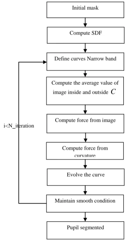
Fig 16: Flowchart of active contour without edges The algorithm illustrated by the flowchart in Figure 16 is based on Chan Vese segmentation algorithm used to separate two objects. One is considered as the foreground and the other as the background. This is a good method to segment two regions statistically different.

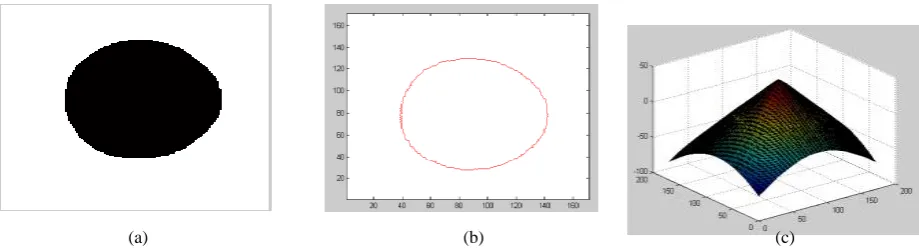
 Initial mask

The mask initialization is the critical step to generate the signed distance function (SDF). The initial mask consists only of two regions: one taken as a background (=0) and the other as the foreground (=1). This mask should be as close as possible to the segmented element in order to reduce thereafter the time computation and solve the problem of active contour sensitivity to the contour initialization. For these reasons we use the edge map (Mask) generated by the image deinoising step of section 3.2 as a first mask.

 Compute SDF



SDF means Signed Distance Function as shown in Figure 17-c. It’s computed from the initial mask (Figure 17-a) using Euclidian distance. By convention [23], the contour Mask

Original Image Image

denoising ComputingROI

Image Thresholding

Eyelashes elimination

(closing)

Maskresizing (opening)

Activecontour withoutedges

Pupilsegmented

Initialmask

DefinecurvesNarrowband

Computetheaveragevalueof

imageinsideandoutside

C

Computeforcefromimage

Computeforcefrom curvature

Evolvethecurve

Maintainsmoothcondition

Pupilsegmented ComputeSDF

iterationNi

_

[image:7.595.58.298.79.380.2]

   



,

,

,



0





x

y

x

y

C



is defined as the intersection

between a plane at the 0 level of



as depicted in Figure

17-b. The moving interface or the contour

C

divides



into two open subsets, where





0

inside

C

and





0

outside. In our work we choose



as an image with real

values because we need to compute distances from the curve

so that the distance function is positive outside

C

and negative inside.

 Define curves Narrowband

The first disadvantage of the level set method is time. It

[image:8.595.61.521.208.332.2]

requires a lot of time to make



change. The solution to this problem is the narrow band approach. The narrow-band algorithm reduces the computation time by restricting the updates to a band of grid points that lies near the level set [19]. Figure 18 gives an example of curves narrow band in which the level curve passes through a set of cells. Only the cells in a neighborhood of the level curve involve their evolution.

Fig 18: A level curve passes through a set of cells.

In our work we define the curves narrow band by the equation (13):

 



 





,

,







,



0

,



1

,



0

,



1



 

13



i

j

i

n

j

m

nB

C







Where

 

i

,

j

is defined as pixel coordinates and

 

n

,

m

the height and width of



.

 Computing the average value of an image inside and outside C

We note the average values of an image inside and outside the

curve

C

by



_inand



_out, respectively:

 

_{ }

14

in

p

in

F

I

in







 

out

p

out

F

I

out







Where,

 











,

,



0

,



0

,



1

,



0

,



1





i

j

i

n

j

m

in

F



 











,

,



0

,



0

,



1

,



0

,



1





i

j

i

n

j

m

out

F



:

in

p

Number of elements of

F

_in.

:

out

p

Number of elements of

F

_out. X

[image:8.595.70.272.526.650.2]

Y

Fig 17: First contour generation. (a) Initial mask. (b) First contour

C

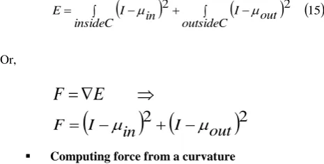
. (c) Signed Distance Function generated from initial mask.

 Computing Force from an image

We used Chan-Vese energy expression to compute the force F from the image I. The well known expression of Chan-Vese energy is given by equation (15):





2 







2

 

15

   outsideC out I insideC in I

E  

Or,







E

F





2





2

out

I

in

I

F













 Computing force from a curvature

In order to compute the curvature we adopted kappa equation which is defined by the following equation [20]:

 

16

2 3 2 2 2 * 2 * 2       _       _{ }  y x xy y x xx y yy x curvature          Where,

2 2 _         _x x  

,

2 2 _         y y





,

         

 2 ₂

x xx  

,

         

 2 ₂

y yy





,

           _xy xy





2

In order to approximate each of the derivatives of



according to x and y, we use the central difference

approximation given by equation (17).The point

P

 

x

,

y

and

their eight neighbor points named



P

up

,

P

down

,

P

left

,

P

right

,

P

upright

,

P

upleft

,

P

downright

,

P

downleft



are

defined in Figure 19.

)

(

)

(

right

P

left

P

x













)

(

)

(

P

_up

down

P

y













 

17

)

(

2

)

(





















right

P

P

left

P

xx









 

P

up

P

down

P

yy













(

)



2

(

)





































upleft

P

downright

P

upright

P

downleft

P

xy











*

25

.

0

*

25

.

0

)

(

*

25

.

0

)

(

*

25

.

0

1



X

X

Y

Y

X

1



X

1



Y

1



Y

P

downright

P

down

P

upleft

P

P

_up

P

_upright

[image:9.595.316.562.71.322.2]

right

P

left

P

downleft

P

Fig 19: Central difference approximation scheme.

 Evolvement of the curve

The value of



after a small time interval



t

was approximated by the first-order Taylor expansion given by equation (18):

 



x

,

y

,

t

t



t

*



_t





 

x

,

y

,

t

  

18













Where:

F

F curvature

t *  _max





 













t

t

max

1

t



is defined by gradient descent and



t

is the time step. The two parameters



and



are defined respectively by the weight of a smoothing term and a coefficient to satisfy Courant, Friedrichs, Lewy (CFL) condition.

The CFL condition is a necessary condition for convergence while solving certain partial differential equations [21]. If this condition is not respected we will produce an incorrect contour as shown in Figure 20.

[image:9.595.54.287.140.258.2]

(a) (b)

[image:9.595.321.542.634.730.2]

 Maintaining a smooth condition of



In order to keep SDF smooth we used the Sussman function [22] defined by equation (19):

   

_{, ,}

 

19

,

1 ,

N j i j i N

j i N

j

i



tS



G













_

Where,

 

_

_{2 2}

_

, 2 ,

,

_

_









_

j i j i j i

S

 

   







   







   







   



























   

  

otherwise

0

0

if

1

-,

max

,

max

0

if

1

-,

max

B

,

A

max

2 2 2

2

2 2 2

-2

,











A

B

C

D

D

C

G

N j i

 

 

A

A

is a matrix that has the positive as well as the negative values of

A

and zero otherwise.

Note_: The other matrix (B, C and D) are manipulated in the same way.



_,

,

0

..

1

0

..

1



, 1

,















_

a

i

n

and

j

m

A



_{i j}



_{i j i j}



_,

,

0

..

1

0

..

1



, ,

1















_

b

i

n

and

j

m

B



_{i j}



_{i j i j}



_,

,

0

..

1

0

..

1



1 ,

,















_

c

i

n

and

j

m

C



_ij



_{ij ij}



_,

,

0

..

1

0

..

1



, 1

,















_

d

i

n

and

j

m

D



_ij



_{ij ij}

4. EXPERIMENTAL RESULTS

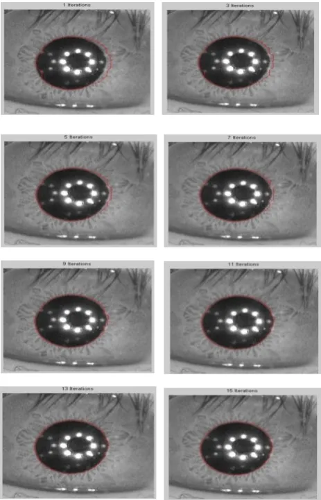
In our algorithm we used a set of parameters to achieve the pupil boundary localization. The parameter used to limit the narrow band border was chosen to , the smoothing parameter , the radius of the largest pupil =75 in the iris database V 3.0 [12], number of image and the number of N_iteration =15 is fixed taking into account the smallest and the largest pupil. These parameters are selected empirically based on the best results of pupil accuracy. We use the eye image in Figure 1 to demonstrate step by step the evolution of the active contour of our method as shown in Figure 21.

In our experiments, we used Matlab 7.9.0 and a computer with a 3 GHz CPU and 1024 Mo of RAM. The CASIA iris image database V3.0 and V1.0 are also used to assess our work. The iris image data base V3.0 includes 2655 each with a size of 280*320.

We take into consideration two important metrics: time computing and accuracy to compare between the three methods: our method, GVF active contour and integro-differential operator.

Table 1 displays the performance of our method of pupil segmentation using CASIA iris image database V1 without corneal reflection removal method because the region of the pupil is artificially filled. Figure 22 shows some samples of detected pupils from CASIA iris image database V1.0. Table 2 shows the performance of the three algorithms: GVF active contour, integro-differential operator and our method using CASIA iris database V3.0. From this table we

accuracy and time computing. Figure 23 shows an example of detected pupils (using a blurred, occluded... iris images) from CASIA iris image database V3.0.

Table 2 shows the performance of the three algorithms: GVF active contour, integro-differential operator and our method using CASIA iris database V3.0. From this table we can deduce that our method gives better matches in terms of accuracy and time computing. Figure 22 shows an example of detected pupils from CASIA iris image database V3.0.

[image:10.595.317.549.184.545.2]

Table 1. Pupil segmentation results for Casia-V1 database using our method without corneal reflection removal

Images

number

Correct Accuracy

CASIA

V1.0

756 756 100%

[image:10.595.311.534.635.724.2]

[image:11.595.46.551.96.670.2]

Table 2. Pupil segmentation accuracy and time of the proposed method using Casia V3.0

Method

Accuracy

(%)

Mean

Time

(s)

Min.

Time

(s)

Max.

Time

(s)

Daugman [10] 95.10 0.78 0.62 0.81

GVF active

contour [10 ]

96.86 0.58 0.40 0.84

Proposed

method

[image:11.595.45.557.507.705.2]

99.62 0.33 0.30 0.44

5. CONCLUSION

Among the biometrics approaches, the iris recognition is known as a good identification system for its high reliability and non evasiveness. In this paper we proposed a novel method for pupil detection used in iris recognition based on Level set method. The first step in our approach is corneal reflection removal, which is useful to eliminate the sources of noise in order to avoid errors in the segmentation stage. This task was achieved in three steps: Image gradient using a white Top-hat, image cleaning and filling corneal reflection points. Then, comes the mask generation stages. This step is efficiently addressed by thresholding and two complement morphological operator closing and opening. Third we precised the pupil boundary localization using namely an active contour without edges. This method is based on the level set technique to deform an initial curve so that it separates the foreground from the background based on the means of the two regions. This kind of active contour is very robust to initialization. The proposed method was tested and evaluated using CASIA V3.0 and V1.0 databases. Some examples were presented to illustrate the results. In this study we compared between three algorithms Daugman, GVF active contour and our approach used for pupil localization. We proved that our method seems to be the fastest and the most accurate compared to those found in literature with an accuracy rates that might reach 100% for CASIA iris image data base V1.0 and 99.62% for CASIA iris image data base V3.0.

6. ACKNOWLEDGMENTS

Authors would like to thank, Iris Recognition Research Group, National Laboratory of Pattern Recognition, Center for Biometrics and Securiy Research, for their collaboration.

REFERENCES

[1] H.-A. Park, K.R. Park, “Iris recognition based on score level

fusion by using SVM”, Pattern Recognition Letters, 28 (2007) 2019-2028.

[2] Y.Adini, Y. Moses, and S. Ullman, “Face recognition: the

problem of compensating for changes in illumination direction”, IEEE Trans. Pattern Anal. Machine Intell. , 19 (1997) 721 - 732.

[3] J. Daugman, “How Iris Recognition Works”, IEEE

Transactions on circuits and systems for video technology, 14 (2004) 21 - 30.

[4] M. Nabti, A. Bouridane, “An effective and fast iris

recognition system based on a combined multiscale”, Pattern Recognition, 41 (2008) 868–879.

[5] R. Wildes, Iris Recognition: “An Emerging Biometric

Technology”, Proceedings of the IEEE, 85 (1997) 1348 - 1363.

[6] L. Masek, “Recognition of human iris patterns for biometric

identification”,The University of Western Australia, 2003.

[7] S. Pundlik,D. Woodard, S. Birchfield, “Non-ideal iris

segmentation using graph cuts”, IEEE Computer Society Conference on Computer Vision and Pattern Recognition Workshops, (2008) 1 - 6.

[8] J. Zuo, N. K. Ratha, J. H. Connell, “A new approach for iris

segmentation”, IEEE Computer Society Conference on

[9] Computer Vision and Pattern Recognition Workshops,

(2008) 1-6.

[10] [9] J. Daugman, “New Methods in Iris Recognition”, IEEE Transactions on systems, man, and cybernetics, 37 (2007)1167-1175.

[11] Z. He, T. Tan, Z. Sun, and X. Qiu, “Toward accurate and fast iris segmentation for iris biometrics”, IEEE Transactions on Pattern analysis and machine intelligence, 31 (2009) 1670 - 1684.

[12] K. Nguyen, C. Fookes, and S. Sridharan, “Fusing shrinking and expanding active contour models for robust iris

segmentation”, 10th International Conference on

Information Science, Signal Processing and their

Applications, (2010) 185 - 188.

[13] A. jarjes, K. Wang and G. J .Mohammed, “GVF snake-based method for accurate pupil contour detection”, Information technology Journal, 9 (2010) 1653-1658.

[14] C. Bastos, I. Tsang and G. Calvalcanti, “A combined pulling & pushing and active contour method for pupil segmentation”, ICASSP (2010).

[15] Z. Zhou and X. Geng, “Projection Functions for Eye Detection”, Pattern Recognition, 37 (2004) 1049-1056.

[16] C. Xu and J.L. Prince, “Snakes, shapes, and gradient vector flow”, IEEE Transactions on image processing, 7 (1998) 359 - 369.

[17] A. Ebrahim Yahya, M. Jan Nordin, “A New Technique for Iris Localization”, International Scientific Conference Computer Science, (2008).

[18] http://www.shawnlankton.com/2007/05/active-contours/, T.F. chan, L.A. Vese , “Active Contours Without Edges”, IEEE TRANSACTIONS ON IMAGE PROCESSING, VOL. 10, NO. 2, FEBRUARY 2001.

[19] http://en.wikipedia.org/wiki/Level_set_method, D. H. Perez, “level set method applied to topology optimization”, grupo de optimizacion structural (GOE), February 2012.

[20] R. Whitaker, “A Level-Set Approach to 3D Reconstruction from Range Data”, the International Journal of Computer Vision, 29 (1998) 203-231.

[21] C. Phillips, “The Level-Set Method”, MIT Undergraduate Journal of Mathematics, (1999).

[22] http://en.wikipedia.org/wiki/Courant%E2%80%93Friedrichs %E2%80%93Lewy_condition, R. Courant, K.O. Friedrichs, H. Lewy, "Ueber die partiellen Differenzgleichungen der mathematische Physik" Math Ann., 100 (1928) pp. 32–74.

[23] M. Sussman, P. Smereka and S. Osher, “A level set approach for computing solutions to incompressible two-phase flow”, University of California, Los Angeles, 14 (1994) 146-159.

[24] S. Lankton, “Sparse Field Methods”, Technical Report, 2009.

[25] W. Aydi, N. Masmoudi, L. Kamoun, “New corneal reflection removal method used in iris recognition system”, World Academy of Science, Engineering and Technology 77 (2011).