Study of Various Decision Tree Pruning Methods with their Empirical Comparison in WEKA

Study of Various Decision Tree Pruning Methods with

their Empirical Comparison in WEKA

Nikita Patel

ME-CSE student, Dept. of Computer Engg. S.P.B. Patel College of Engineering,

Linch, Mehsana, Gujrat, India

Saurabh Upadhyay

Associate Prof., Dept. of Computer Engg. S.P.B. Patel College of Engineering,

Linch, Mehsana, Gujrat, India

ABSTRACT

Classification is important problem in data mining. Given a data set, classifier generates meaningful description for each class. Decision trees are most effective and widely used classification methods. There are several algorithms for induction of decision trees. These trees are first induced and then prune subtrees with subsequent pruning phase to improve accuracy and prevent overfitting. In this paper, various pruning methods are discussed with their features and also effectiveness of pruning is evaluated. Accuracy is measured for diabetes and glass dataset with various pruning factors. The experiments are shown for this two datasets for measuring accuracy and size of the tree.

General Terms

Keywords

Attribute Selection Measures, Decision tree, Post pruning, Pre pruning.

1.

INTRODUCTION

Data mining is the extraction of hidden predictive information from large databases [2]. It is a powerful new technology with great potential to help companies focus on the most important information in their data warehouses. Data mining is actually part of the knowledge discovery process. The Knowledge Discovery in Databases [2] process comprises of a few steps leading from raw data collections to some form of new knowledge. Classification in data mining find a model for class attribute as a function of the values of other attributes. Classifier generates meaningful description for each class that are used to classify instances of the given dataset [1]. To Classifying credit card transactions as legitimate or fraudulent is an example of classification. There are several approaches for the classification like neural network, SVM, decision tree etc. In this paper decision tree is illustrated as classifier.

Decision tree is flow like structure [2]. Decision tree induction is the top down process. At the top the root is selected using some attribute selection measures like information gain, gain ratio, gini index etc. During induction of the tree attribute is selected by this attribute selection measures [2]. Although decision tree is induced by various algorithms, but sometimes it happens that it generates unwanted & meaningless rules as it grows deeper, it is called overfitting. Pruning is needed to avoid large tree or problem of overfitting [1]. Pruning means reducing size of the tree that are too larger and deeper. The problem of noise and overfitting reduces the efficiency and accuracy of data.

There are two types of the pruning, pre pruning and post pruning. First is Post pruning, in which the tree is build first and then reduction of branches & levels of the decision tree is

done. Second is Pre pruning, in which while building the decision tree keep on checking whether tree is overfitting. There are no of methods for post pruning like reduced error pruning, Error complexity pruning, minimum Error pruning, cost based pruning etc. These all methods are discussed in later sections. Two technique for pre pruning are there: minimum no of obj pruning and chi square pruning. Two data sets are taken for experiments in weka tool. There are various decision tree induction algorithm and various pruning parameters like confidence factor , minimum no of objects(at leaf node), num of folds of given data set.

In section 2 classifications and various approaches and its applications are discussed. This section illustrates various approaches for the classification with their features. Section 3 gives detail of decision tree with various attribute selection measures for inducing decision tree. In section 4 post pruning and pre pruning techniques are discussed with their methods. Section 5 evaluates results of Diabetes and Glass dataset with various pruning factors in weka interface like confidence factor, Minimum no of objects, No of folds (reduced error pruning). Accuracy and size of the tree measured for both data sets. Section 6 represents concluding remarks.

2.

CLASSIFICATION & VARIOUS

APPROCHES

Classification [1] has been studied extensively by the machine learning community as a possible solution to the knowledge acquisition or knowledge extraction problem

2.1

What is Classification?

Classification is the task of generalizing known structure to apply to new data. For example, an e-mail program might attempt to classify an e-mail as "legitimate" or as "spam". Data classification [2] is a two step process. First step is Learning, which consist of analysis of training data by a classification algorithm then after learned model or classifier is represented in the form of classification rules [3].Second step is Classification, in which Test data are used to estimate the accuracy of the classification rules.

2.2

Application

2.3

Approaches

There are various approaches used for the classification. Any classification method uses a set of features or parameters to characterize each object, where these features should be relevant to the task at hand. We consider here methods for supervised classification, meaning that a human expert both has determined into what classes an object may be categorized and also has provided a set of sample objects with known classes.

2.3.1

Decision tree

Decision Tree [2] is a flowchart like tree structure. The decision tree consists of three elements, root node, internal node and a leaf node. Top most element is the root node. Leaf node is the terminal element of the structure and the nodes in between is called the internal node. Each internal node denotes test on an attribute, each branch represents an outcome of the test, and each leaf node holds a class label. The decision tree is constructed based on "Divide and Conquer" [5]. That is the tree is formed by framing rules which will branch out from the nodes and sub-nodes until the decision is made. There are different methods of forming the decision rules for Decision Trees. The nodes are selected from the top level based on quality attributes such as Information Gain, Gain Ratio, Gini Index etc. The C4.5 Decision tree uses Gain Ratio to construct the tree, the element with highest gain ratio is taken as the root node and the dataset is split based on the root element values. Again the information gain is calculated for all the sub-nodes individually and the process is repeated until the prediction is completed.

2.3.2

Neural Networks

Neural Network consist of three layer, that are input layer, hidden layer and output layer [5].Multilayer Perceptron (MLP) is a neural network based algorithm. At the input layer nodes(neurons) define the input values. The probabilities of inputs are assigned weights before given to the neurons in the hidden layer. Greater the weight, the neuron favors the result. Finally the neurons in the output layer represent the outcome. Neural networks can be applied to any situation virtually provided that relationship exists between the input and the output. The neurons contain activation function through which the signal is passed to predict the output. There are two types of trainings used in neural networks, supervised and unsupervised training. The supervised training algorithm generally used for MLP is back-propagation algorithm. Back propagation algorithm is where the predicted value is compared with the actual value andif the mean squared error is more, the process is repeated again until the mean squared error is minimized [6].

2.3.3

SVM

Support Vector Machine [2] is a promising new method for the classification. It uses a nonlinear mapping to transform original data into a higher dimension. Within this dimension it searches for the linear optimal separating support decision boundary. The SVM finds this hyper plane using essential training tuples and margins. Support vector machines (SVMs) were originally designed for binary classification [7].SVM classifies both linearly separable data and linearly inseparable data. The SVM for the linearly separable data does not give feasible solution. But SVM for the linearly inseparable data are capable of finding nonlinear decision boundaries.

3.

DECISION TREE AS CLASSIFIER

Decision tree Induction is top down approach which starts from the root node and explore from top to bottom. There are various algorithms that are used for building the decision tree. Basic algorithm for constructing decision tree is as follows: first tree is constructed in a Top down recursive divide and conquer method. At start all the training examples are at root then after examples are partitioned recursively based on the selected attribute [8]. ID3 algorithm determines ID3 heuristic. It splits attribute based on their entropy. TDIDT algorithm constructs a set of classification rules via the intermediate representation of a decision tree [9,10].Weka interface [11] can be used for testing data sets using a variety of open source machine learning algorithms. The data sets were tested using the J48 decision tree inducing algorithm and then after the result is visualized for decision tree. As discussed earlier, decision tree is induced by the quality attributes such as information gain, gain ratio, gini index etc. These all attribute selection measures are described as follow.

3.1

Attribute Selection Measures

Attribute selection is the process of removing the redundant attributes that are deemed irrelevant to the data mining task [12].The objective of attribute selection is therefore to search for a worthy set of attributes that produce comparable classification results to the case when all the attributes are used. Measures for selecting the best split attributes are almost all defined in terms of the reduction of impurity from parent to child node(before splitting)[13].The larger the reduction of impurity, the better the selected split attribute. There are number of attribute selection measures are exist. Let t, be a training set of class labelled tuples. Suppose the class label has c distinct values defining c distinct classes.

3.1.1

Information Gain

Information gain measures the expected reduction in entropy caused by partitioning the examples according to attribute.ID3 uses information gain as its attribute selection measure. This is based on Shannon’s entropy.

Where Info(D) is also known as entropy of D.

3.1.2

Gain Ratio

Information gain measure is biased toward tests with many outcomes. Therefore the information gained by partitioning on attribute is maximal, such a partitioning is useless for classification.C4.5, a successor of ID3 [2] uses an extension to the information gain known as Gain ratio.

Where Gain(A) is expected reduction in the information requirement caused by knowing the value of A(attribute).

(D)

3.1.3

Gini Index

Gini index is used in CART. Gini index measures the impurity of D, a data partition or set of training tuples as

Where Pi is the probability that a tuple in D belongs to the class Ci.

4.

PRUNING METHODS FOR

DECISION TREE

Although the decision tree generated by the ID3,C4.5 are accurate and efficient, but they often provide very large trees that make them incomprehensible to the experts[8]. When decision tree induced, many of the branches will reflect anomalies in the training data due to noise. This problem of overfitting happens when the learning algorithm continues to develop hypotheses that reduce training set error at the cost of an increased test set errors. To overcome these problem of overfitting, pruning is necessary. Pruning a decision tree is a fundamental step in optimizing the computational efficiency as well as classification accuracy. Pruning usually results in reducing size of tree, avoids unnecessary complexity, and to avoid overfitting of the data sets when classifying new data. Overfitting can lead to an excessively large number of rules, many of which have very little predictive value for unseen data[14]. There are two techniques for pruning pre-pruning and post-pruning, which are discussed next in this paper.

4.1

Post-pruning

Post-pruning is also known as backward pruning. In this, first Generate the decision tree and then remove non-significant branches. Post-pruning a decision tree implies that we begin by generating the (complete) tree and then adjust it with the aim of improving the classification accuracy on unseen instances. There are two principal methods of doing this. One method that is widely used begins by converting the tree to an equivalent set of rules. Another commonly used approach aims to retain the decision tree but to replace some of its subtrees by leaf nodes, thus converting a complete tree to a smaller pruned one which predicts the classification of unseen instances at least as accurately. There are various methods for the post pruning.

4.1.1

Reduced Error Pruning

This method was proposed by Quinlan [8]. It is simplest and most understandable method in decision tree pruning. This method considers each of the decision nodes in the tree to be candidates for pruning, consist of removing the subtree rooted at that node, making it a leaf node. The available data is divided into three parts: the training examples, the validation examples used for pruning the tree, and a set of test examples used to provide an unbiased estimate of accuracy over future unseen examples. If the error rate of the new tree would be equal to or smaller than that of the original tree and that subtree contains no subtree with the same property, then subtree is replaced by leaf node, means pruning is done. Otherwise don’t prune it. The advantage of this method is its linear computational complexity [15].When the test set is much smaller than the training set, this method may lead to over pruning. Many researchers found that Reduced Error Pruning performed as well as most of the other pruning

methods in terms of accuracy and better than most in terms of tree size [15].

4.1.2

Error complexity pruning

In error complexity pruning is concern with calculating error cost of a node. It finds error complexity at each node. the error cost of the node is calculated using following equation:

Where:

r(t) is error rate of a node which is given as:

p(t) is probability of occurrence of a node

If node t was not pruned then error cost of subtree T, rooted at t:

The error complexity of the node is given as:

a: measures the VALUE of corresponding subtree.

The method consists of following steps:

 a is computed for each node.  the minimum a node is pruned.

 the above is repeated and a forest of pruned tree is formed.

 the tree with best accuracy is selected.

4.1.3

Minimum Error pruning

This method was developed by Niblett and Brotko [16]. It is a bottom-up approach which seeks a single tree that minimizes the expected error rate on an independent data set. If it is predicted that all future examples will be in class c, the following equation is used to predict the expected error rate of pruning at node t:

Where:

k=no of class,

nt=no of examples in node t

nt,c=no of examples assigned to class c in node t

 At each non leaf node in the tree, calculate expected error rate if that subtree is pruned.

 Calculate the expected error rate for that node if subtree is not pruned.

 If pruning the node leads to greater expected error rate, then keep the subtree; otherwise, prune it.

4.1.4

Cost based pruning

This is one of the post pruning technique. In this method not only an error rate is considered at each node but also a cost is considered. That is for pruning decision tree error rate and cost of deciding selection of one or more class-label attribute is considered. Here one example is explained for healthy or sick classification [20]. Two type of pruning is shown error pruning and cost based pruning:

Fig 1. Example of cost based pruning [20]

Left side of the figure shows that the subtree should be pruned by error-minimization algorithms because the number of errors stays the same (5/100) if the subtree is pruned to a leaf. Right side of the figure illustrates the reverse situation which is cost based pruning. Not by loss-minimization algorithms with a 10 to 1 loss for classifying sick as healthy against vice-versa. The right tree shows the opposite situation where error minimization algorithms should not prune, yet loss minimization with a 10 to 1 loss should prune since both leaves should be labelled "sick."

4.2

Pre-pruning

Pre-pruning is also called forward pruning or online-pruning. Pre-pruning prevent the generation of non-significant branches. Pre-pruning a decision tree involves using a ‘termination condition’ to decide when it is desirable to terminate some of the branches prematurely as the tree is generated. When constructing the tree some significant measures can be used to assess the goodness of a split. If partitioning the tuples at a node would result the split that falls below a prespecified threshold, then further partitioning of the given subset is halted otherwise it is expanded. High threshold result in oversimplified trees, whereas low threshold result in very little simplification. There are various approaches for the pre-pruning.

4.2.1

Minimum no of object pruning

In this method of pruning, the minimum no of object is specified as a threshold value. In weka interface [11], there is one parameter in J48 (weka implementation of C4.5), called minobj is set to specify threshold value. Whenever the split is made which yields a child leaf that represents less than minobj from the data set, the parent node and children node are compressed to a single node. The different ranges of the minimum no of objects are set for few examples and tested for accuracy. To access the performance on sample domains, a series of both training and testing sets were sent through a decision tree created by J48 algorithm [11].This is shown in Experiments in next section of this paper. It is shown that

although increasing no of objects simplifies the tree, but it reduces accuracy of the dataset.

Fig 2:Minnumobj pruning in weka, replacing children node with parent [11]

As shown in figure, minnumobj is specified as 30, so when inducing the tree at last it finds 34 and 9. 34>30, so it is greater than this threshold value and node is not spitted (pruning is done).

4.2.2

Chi-square pruning

This approach to pruning is to apply a statistical test[18] to the data to determine whether a split on some feature Xk is statistically significant, in terms of the effect of the split on the distribution of classes in the partition on data induced by the split. Here null hypothesis is considered, that the data is independently distributed according to a distribution on data consistent with that at the current node [19]. If this null hypothesis cannot be rejected with high probability, then the split is not adopted and ID3 is terminated at this node. It is based only on the distribution of classes induced by the single decision of splitting at the node and not by the decisions made as a result of growing a full subtree below this node as in the case of post pruning. So here null hypothesis is stated as: feature Xk is unrelated to the classification of data given features already branched on before this node. This is the hypothesis that we form to determine whether or not to reject the split. The split is only accepted if this null hypothesis can be rejected with high probability. We can perform chi-squared test as:

According to this equation one contingency table is generated and according to this values .

Consider one example, The statistical for Pearson’s chi-square test [19], which will be used here as a test of independence. To think about this, suppose that at the current node the data is split 10:10 between negative and positive examples. Further more, suppose there are 8 instances for which Xk is false, and 12 for which Xk is true. We’d like to understand whether a split that generates labeled data 3:5 (on the Xk false branch) and 7:5 (on the Xk true branch) could occur simply by chance.

5.

EXPERIMENTS, RESULTS &

DISCUSSION

minNumobj in weka specifies minimum no of objects(instances) at the leaf node. That is when decision tree is induced, at every split it will check minimum no of object at leaf. If instances at leaf are greater than minimum num of obj then pruning is done. NumFold parameter in weka is affected only when reduced error pruning parameter is true. That is this parameter determines amount of data used for reduced error pruning. Among numFolds one fold is used for pruning and rest of them for growing the tree. Suppose numFold is 3 then 1 fold is used for pruning and 2 fold for training for growing the tree.

Experiments on weka shows the accuracy and size of tree for particular parameter. Here size of tree is considered because it is mainly concerned with pruning. It indicates with pruning how accuracy(increasing or decreasing) is get. Below graph shows measure for accuracy and size of tree for both data sets in weka.

Fig 3: Minnumobj vs Accuracy

Fig 3 and Fig 4 shows comparision of both data sets for the accuracy & size of tree when minNumobj parameter is used. Whenever minnumobj is increased accuracy is almost same but tree size is changed. At starting it seems to be increasing, but as minnumobj is more increased , size of tree is decreased means more pruning is done and accuracy is almost same.

Fig 4: Minnumobj vs Size of tree

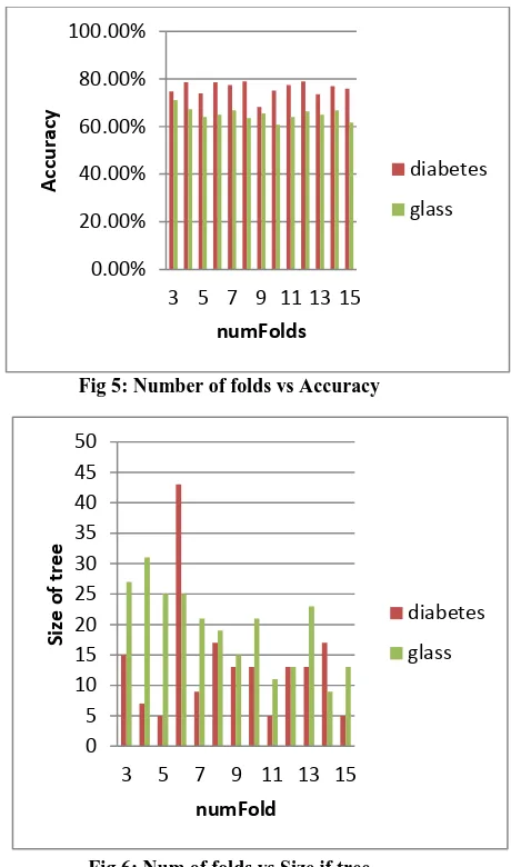
Fig 5: Number of folds vs Accuracy

Fig 6: Num of folds vs Size if tree

Fig 5 and Fig 6 shows comparision of accuracy and size of tree for both data set when numFold parameter is used. For reduced error pruning numFold is used. Whenever num of folds are increased accuracy for both datasets almost increases, but here it can’t be perfect train for size of the tree. For Diabetes dataset size of the tree suddenly increases for values between 5 to 6. For Glass dataset it is almost increases at starting, but as the num of folds increasing more size of tree reduces and accuracy is almost same.

6.

CONCLUSION

In this paper, various pruning algorithms are discussed. In post pruning, first decision tree is induced and then after it is pruned where as in pre pruning; nodes are not expanded during the building phase. As a result, fewer nodes are expanded during the building phase, and thus the complexity of constructing the decision tree is reduced. Post pruning and pre pruning algorithms shows accuracy against pruning. In pre pruning chi square test is performed. This test is related to statistical measurements. Accuracy and tree length are measured for various pruning factors for large data sets. The experiments for diabetes and glass data set, when confidence factor is increased accuracy is almost constant but size of the tree is increased so it doesn’t seems to be effective. Second pruning parameter is minimum no of obj. When minobj is increases accuracy is almost increases and size of the tree is almost decreases. No of fold is one pruning parameter in weka, which affected only when reduced error pruning is true.

0.00% 20.00% 40.00% 60.00% 80.00% 100.00%

5 10 15 20 25 30

A

cc

u

rac

y

minNumobj

diabetes

glass

0 5 10 15 20 25 30 35

5 10 15 20 25 30

Si

ze

o

f tr

e

e

minNumobj

diabetes

glass

0.00% 20.00% 40.00% 60.00% 80.00% 100.00%

3 5 7 9 11 13 15

A

cc

u

rac

y

numFolds

diabetes

glass

0 5 10 15 20 25 30 35 40 45 50

3 5 7 9 11 13 15

Si

ze

o

f tr

e

e

numFold

diabetes

When no of fold increases, accuracy almost increases and size of tree sometimes reduced.

7.

REFERENCES

[1] Dipti D. Patil, V. M. Wadhai, J. A. Gokhale, “Evaluation of Decision Tree Pruning Algorithms for Complexity and Classification Accuracy”,IJCSE,volume-II.

[2] Jiawei Han, MichelineKamber, “Data Mining Concepts and Techniques”, pp. 279-328, 2001.

[3] Tom. M. Mitchell, “Machine Learning”, McGraw-Hill Publications, 1997

[4] “Application of Data Mining Techniques for Medical Image Classification” Proceedings of the Second International Workshop on multimedia Data Mining(MDM/KDD’2001) in conjuction with ACM SIGKDD conference. San Francisco,USA,August 26,2001.

[5] Cscu.cornell.edu, 2003 [Online] SimonaDespa, 4 March 2003

Retrievedfromhttp://www.cscu.cornell.edu/news/statnew s/stnews55.pdf [Accessed on May 5, 2009]

[6] Fu, L. (1994). "Rule generation from neural networks." IEEE Transactions on Systems, Man and Cybernetics 24(8): 1114-1124.

[7] Chih-Wei Hsu ,“A comparison of methods for multiclass support vector machines”,Neural Network ,IEEE transaction on mar 2002.

[8] J. Quinlan,” Simplifying decision trees”, Int. J. Human-Computer Studies.

[9] J.R. Quinlan, “C4.5: programs for Machine Learning”, Morgan Kaufmann, New York,1993

[10]J.R. Quinlan, “Induction of Decision Trees”, Machine Learning 1(1986) pp.81-106.

[11]SamDrazin and Matt Montag,”Decision Tree Analysis using Weka”, Machine Learning-Project II, University of Miami.

[12]K.C. Tan, E.J. Teoh, Q. Yu, K.C. Goh,” A hybrid evolutionary algorithm for attribute selection in data mining”, Department of Electrical and Computer Engineering, National University of Singapore, 4 Engineering Drive 3, Singapore 117576, Singapore.Rochester Institute of Technology, USA.

[13]Liangxiao JIANG, Chaoqun LI,” An Empirical Study on Attribute Selection Measures in Decision Tree Learning”, Journal of Computational Information Systems6:1(2010) 105-112.

[14]Max Bramer,” Pre-pruning Classification Trees to Reduce Overfitting in Noisy Domains”, Faculty of Technology, University of Portsmouth, UK.

[15]F. Esposito, D. Malerba, and G. Semeraro,”A comparative Analysis of Methods for Pruning Decision Trees”, IEEE transactions on pattern analysis and machine intelligence,19(5): pp. 476-491, 1997.

[16]B. Cestnik, and I. Bratko, ”Estimating Probabilities in Tree Pruning”, EWSL, pp. 138-150, 1991.

[17]Esposito F., Malerba D., Semeraro G,”A Comparative Analysis of Methods for Pruning Decision Trees”, IEEE Transactions on Pattern Analysis and Machine Intelligence, VOL. 19, NO. 5, 1997, P. 476-491.

[18]Minhaz Fahim Zibran,” CHI-Squared Test of Independence”, Department of Computer Science,University of Calgary, Alberta, Canada.

[19]David C. Howell,” Chi-square test Analysis of Contingency tables”, University of Vermont.