A Penalty Function Algorithm with Objective Parameters and Constraint Penalty Parameter for Multi Objective Programming

http://dx.doi.org/10.4236/ajor.2014.46032

A Penalty Function Algorithm with

Objective Parameters and Constraint

Penalty Parameter for Multi-Objective

Programming

Zhiqing Meng, Rui Shen, Min Jiang

College of Business and Administration, Zhejiang University of Technology, Hangzhou, China Email: [email protected],

[email protected]

, [email protected],

Received 28 August 2014; revised 22 September 2014; accepted 6 October 2014

Copyright © 2014 by authors and Scientific Research Publishing Inc.

This work is licensed under the Creative Commons Attribution International License (CC BY). http://creativecommons.org/licenses/by/4.0/

Abstract

In this paper, we present an algorithm to solve the inequality constrained multi-objective pro-gramming (MP) by using a penalty function with objective parameters and constraint penalty pa-rameter. First, the penalty function with objective parameters and constraint penalty parameter for MP and the corresponding unconstraint penalty optimization problem (UPOP) is defined. Un-der some conditions, a Pareto efficient solution (or a weakly-efficient solution) to UPOP is proved to be a Pareto efficient solution (or a weakly-efficient solution) to MP. The penalty function is proved to be exact under a stable condition. Then, we design an algorithm to solve MP and prove its convergence. Finally, numerical examples show that the algorithm may help decision makers to find a satisfactory solution to MP.

Keywords

Multi-Objective Programming, Penalty Function, Objective Parameters, Constraint Penalty Parameter, Pareto Weakly-Efficient Solution

1. Introduction

formulation to interactive multiobjective programming problems. Ruan and Huang [4] studied weak calmness and weak stability of exact penalty functions for multiobjective programming. By penalty function, Liu [5]

derived necessary and sufficient conditions without a constraint qualification for e-Pareto optimality of multi- objective programming, and the generalized e-saddle point for Pareto optimality of the vector Lagrangian. Huang and Yang [6] gave nonlinear Lagrangian for multiobjective optimization to duality and exact penalization. Chang and Lin [7] solved interval goal programming by using S-shaped penalty function. Antczak [8] studied the vector exact l₁ penalty method for nondifferentiable convex multiobjective programming problems. Huang, Teo and Yang [9] discussed calmness of exact penalization in vector optimization with cone constraints. Huang

[10] proved calmness of exact penalization in constrained scalar set-valued optimization. Meng, Shen and Jiang

[11] defined an objective penalty function based on objective weight for multiobjective optimization problem and presented an interactive algorithm. This paper defines a penalty function with objective parameters and constraint penalty parameter which differs from an objective penalty function in [11].

Because it is almost not possible for decision makers (DMs) to obtain all efficient solutions to MP, it is significant to present an efficient algorithm of MP so that DMs finds an easy and satisfactory solution to the MP. Luque, Ruiz and Steuer pointed out that an efficient algorithms not only help decision makers learn more about efficient solutions, but also navigate to a final solution as quickly as possible [12]. This paper presents an algorithm by modifying every objective parameter of penalty function so that a final solution is easily and quickly obtained. In Section 2, we introduce a penalty function with the objective parameters and constraint penalty parameter, and its algorithm. In Section 3, we give numerical results to show that the proposed algorithm is efficient.

2. Penalty Function with Objective Parameters and Constraint Penalty Parameter

In this paper we consider the following inequality constrained multi-objective programming:

(

)

( )

(

( ) ( )

( )

)

( )

1 2

MP min , , ,

s.t. 0, 1, 2, , ,

q i

f x f x f x f x

g x i m

=

≤ =



 (1)

where 1

{ }

1

{ }

: n , : n

j i

f R →R  +∞ g R →R  +∞ , for j∈ =J

{

1, 2,,q

}

,i∈ =I

{

1, 2,,m

}

.

We denote the feasible set of MP (1) by X =

{

x∈R g xn i

( )

≤0,i∈I

}

. As usual, x∈X is called a Pareto

weakly-efficient solution if there is no x∈X such that f_j

( )

x < f_j

( )

x for all j∈J, i.e. f x

( )

< f x

( )

. x∈X is called a Pareto efficient solution if there is no x∈X such that f_j

( )

x ≤ f_j

( )

x for all j∈J and

( )

( )

j j

f x < f x for at least one j∈J, i.e. f x

( )

 f x

( )

.

Let functions Q R: →R

{ }

+∞ and P R: →R

{ }

+∞ satisfy

( )

( )

( )

2

( )

1 2 1

0 if and only if 0 0 if and only if 0

if and only if 0

Q t t

Q t t

Q t Q t t t

= ≤

 

> >



 _{> > >}



where lim

( )

0

t→−∞Q t = and

( )

( )

( )

2

( )

1 2 1

0 if and only if 0, 0 if and only if 0

if and only if 0.

P t t

P t t

P t P t t t

= ≤

 

> >



 _{> > >}

 Let

(

, ,

)

(

( )

)

(

( )

)

, 1, 2, , ,

j j j j i

i I

F x M ρ Q f x M ρ P g x j q

∈

= − +

∑

= 

where Mj

(

j=1, 2,,q

)

is an objective parameter and ρ >0 is the constraint penalty parameter. Let

(

M M1, 2, ,Mq

)

=

(

x, ,ρ

)

=

(

F x M1

(

, 1,ρ

) (

,F2 x M, 2,ρ

)

, ,Fq

(

x M, q,ρ

)

)

.

F M 

Consider the following unconstraint penalty optimization problem:

(

)

(

)

MP M,ρ minF x,M,ρ , s t. . x∈Rn.

For x∈Rn, let index set

(

)

{

(

)

}

0

, , _j , _j, 0, for ,

J x M ρ = j∈J F x M ρ = j∈J

(

, ,

)

{

j

(

, j,

)

0, for

}

.

J+ x M ρ = j∈J F x M ρ > j∈J

We have J=J0

(

x,M,ρ

)

J+

(

x,M,ρ

)

.

Theorem 1. Suppose that for given

(

M,

ρ

)

, x_M* is a Pareto weakly-efficient solution to MP

(

M,

ρ

)

. Then the following three assertions hold:

1) If 0

(

*

)

, ,

M

J x M ρ ≠ ∅, then x_M* is a feasible solution to (MP),

( )

*

j M j

f x ≤M for all 0

(

*

)

, ,

M

j∈J x M ρ and f_j

( )

x*_M >M_j for all j∈J+

(

x*_M,M,ρ

)

.

2) If J0

(

x*_M,M,ρ

)

= ∅ ( i.e. F

(

x_M*,M,ρ

)

>0), then there is no x∈X such that f x

( )

< f x

( )

*_M . 3) If F

(

x*_M,M,ρ

)

>0 and x*_M is a feasible solution to (MP), then x*_M is a Pareto weakly-efficient solution to (MP).

Proof. 1) The conclusion is obvious from the definitions of P and Q. 2) Suppose that there be an x∈X such that

( )

( )

*

M

f x < f x . When

( )

*

j M j

f x ≤M for some j∈J, we have

( )

(

)

(

( )

*

)

(

( )

*

)

(

( )

*

)

1

.

m

j j j M j j M j i M

i

Q f x M Q f x M Q f x M ρ P g x

=

− = − < − +

∑

When

( )

*

j M j

f x >M for some j∈J, we have

( )

(

)

(

( )

*

)

(

( )

*

)

(

( )

*

)

1

.

m

j j j M j j M j i M

i

Q f x M Q f x M Q f x M ρ P g x

=

− < − ≤ − +

∑

Hence,

(

_{, ,}

)

(

* _{, ,}

)

M

x ρ < x ρ

F M F M , then x*_M is not a Pareto weakly-efficient solution to MP

(

M,

ρ

)

. 3) According to 2), the conclusion holds.

Theorem 2. Suppose that for a given

(

M,

ρ

)

, x_M* is a Pareto efficient solution to MP

(

M,

ρ

)

. Then the following three assertions hold:

1) If J0

(

x_M* ,M,ρ

)

≠ ∅, then xM* is a feasible solution to (MP),

( )

*

j M j

f x ≤M for all j∈J0

(

x*_M,M,ρ

)

and f_j

( )

x*_M >M_j for all j∈J+

(

x*_M,M,ρ

)

.

2) If 0

(

*_{, ,}

)

M

J x M ρ ≠ ∅ ( i.e.

(

* _{, ,}

)

₀

M

x ρ >

F M ), then there is no x∈X such that

( )

( )

*

M

f x  f x . 3) If

(

* _{, ,}

)

₀

M

x ρ >

F M and x*_M is a feasible solution to (MP), then x*_M is a Pareto efficient solution to (MP).

Proof. 1) The conclusion is obvious from the definitions of P and Q. 2) Suppose that there be an x∈X such that

( )

( )

*

M

f x f x . When

( )

*

j M j

f x ≤M for some j∈J, we have

( )

(

)

(

( )

*

)

(

( )

*

)

(

( )

*

)

1

.

m

j j j M j j M j i M

i

Q f x M Q f x M Q f x M ρ P g x

=

− = − < − +

∑

When

( )

*

j M j

( )

(

)

(

( )

*

)

(

( )

*

)

(

( )

*

)

1

.

m

j j j M j j M j i M

i

Q f x M Q f x M Q f x M ρ P g x

=

− _ − _ − +

∑

Hence, F

(

x,M,ρ

)

F

(

x*_M,M,ρ

)

, then x_M* is not a Pareto efficient solution to MP

(

M,

ρ

)

. 3) According to 2), the conclusion holds.

Based on Theorem 1, we develop an algorithm to compute an efficient solution to (MP). The algorithm solves the problem MP

(

M,

ρ

)

sequentially, and is called Multiobjective Penalty Function Algorithm (MPFA for short).

MPFA Algorithm:

Step 1: Choose x0∈X , ρ >₁ 0, N>1 and *j min j

( )

x X

M f x

∈

< for each j∈J. Let k=1, and

( )

₍

₎

* 0 1 2 j j j

M f x

M = + j∈J .

Step 2: Solve min

(

, ,

)

n

k k x R

x ρ

∈ F M , where

(

1, 2, ,

)

k k k k

q

M M M

=

M  . Let k

x be a Pareto weakly-efficient solution.

Step 3: If 0

(

k_, k_,

)

k

J x M ρ ≠ ∅, for each j∈J, let

* 1 2 k j j k j M M

M + = + , ρk+₁ =Nρk,k+ =1: k and go to

Step 2. Otherwise, F

(

xk,M_k,ρ_k

)

> 0, go to Step 4.

Step 4: If xk is not feasible to (MP), for each j∈J, let

* 1 2 k j j k j M M

M + = + , ρk+₁=Nρk,k+ =1: k and go

to Step 2. Otherwise, stop and xk is a Pareto weakly-efficient solution to (MP). In the MPFA algorithm, it is assumed that for each j∈J *

( )

min

j j

x X

M f x

∈

< can always be obtained . The convergence of the MPFA algorithm is proved in the following theorem. For some j∈J, let

(

, _j

)

{

k

(

_j

( )

k k_j

)

, 1, 2,

}

,

S L f = x L≥Q f x −M k= 

which is called a Q-level set. S L f

(

, _j

)

is bounded if, for any given L>0 and a convergent sequence

*

k

j j

M →M , S L f

(

, _j

)

is bounded.

Theorem 3. Suppose that Q, f_j

(

j∈J

)

and g_i

(

i∈I

)

are continuous on Rn, and the Q-level set

(

, _j

)

S L f is bounded for all j∈J. Let

{ }

xk be the sequence generated by the MPFA algorithm.

1) If

{ }(

xk k=1, 2,,k

)

is a finite sequence (i.e., the MPFA algorithm stops at the k-th iteration), then k

x is a Pareto weakly-efficient solution to (MP). 2) If

{ }

k

x is an infinite sequence, then

{ }

k

x is bounded and any limit point of it is a Pareto weakly- efficient solution to (MP).

Proof. For all j∈J, it is clear that the sequence

{ }

k j

M decreases with

* 1 *

, 1, 2, .

2 k j j k j j M M

M + −M = − k=  (2) Therefore,

{ }

k

j

M converges to M*_j for all j∈J.

1) If the MPFA algorithm terminates at the kth iteration and the second situation of Step 4 occurs, by Theorem 1, xk is a Pareto weakly-efficient solution to (MP).

2) We first show that the sequence

{ }

xk is bounded. From the MPFA algorithm, we have M*_j < f_j

( )

x for all x∈X . Since

{ }

k

j

M converges to *

j

M for all j∈J, there is a k′ such that k

( )

j j

M < f x for all x∈X and all k>k′. If k

x ∈X for each k>k′, we have

(

( )

k k

)

0

j j

have

(

k, ,

)

0

k k

x ρ >

F M for all k>k′. By Theorem 1, there is a j∈J such that

( )

k

( )

0 _{, 1, 2, .}

j j

f x ≤ f x k= +k′ k′+ 

So,

( )

(

)

(

( )

0

)

, 1, 2, .

k k k

j j j j

Q f x −M ≤Q f x −M k= +k′ k′+ 

Therefore, there is an L>0 such that

( )

(

)

(

( )

0

)

, 1, 2, .

k k k

j j j j

Q f x −M ≤Q f x −M <L k= 

Since S L f

(

, _j

)

is bounded, the sequence

{ }

k

x is bounded. Without loss of generality, we assume

*

k

x →x . Since xk is a Pareto weakly-efficient solution to MP

(

Mk,ρ_k

)

, for some j, there are infinite

k>k′ such that

( )

(

)

(

( )

)

(

( )

0

)

1

.

m

k k k k

j j k i j j

i

Q f x M ρ P g x Q f x M

=

− +

∑

≤ −

We have

( )

(

)

(

( )

0

)

(

( )

)

1

1

.

m

k k k k

i j j j j

i k

P g x Q f x M Q f x M

ρ =

 

≤ _ − − − _

∑

When ρ → +∞_k , we have

(

( )

*

)

1

0

m

i i

P g x

=

=

∑

. Hence, x*∈X . If x* is not a Pareto weakly-efficient

solution to (MP), there is an x∈X such that

( )

( )

*

f x < f x . Let

{

( )

*

( )

}

min fj x fj x j 1, 2, ,q

δ = − =  .

From k *

x →x , there is some k such that

( ) ( )

* k

( )

*

( )

_{, 1, 2, , .}

j j j j

f x − f x < ≤δ f x − f x j=  q

So, we have _{f x}

( )

_{< f x}

( )

k _{, which by Theorem 1 is a contradiction. Hence,} *

x is a Pareto weakly-efficient solution to (MP).

Theorem 3 means that the MPFA algorithm is convergent in theory. Now, we discuss the exactness of the penalty function for (MP). If there are an M′∈Rq and ρ′ such that a Pareto weakly-efficient solution x* to (MP) is also a Pareto weakly-efficient solution to

(

P

(

M,ρ

)

)

for ∀M <M′ and ∀ >ρ ρ′, then

(

x, ,

ρ

)

F M is called an exact penalty function.

Let (MP(s)) be a perturbed problem of (MP) given by

( )

(

)

( )

(

( ) ( )

( )

)

( )

1 2

MP min , , ,

s.t. , 1, 2, , ,

q

i i

s f x f x f x f x

g x s i m

=

≤ =



 (3) where s=

(

s s₁, ₂,,s_m

)

. Similar to that for a constrained penalty function in [12], we define stability.

Definition 1. Let x be any feasible solution to (MP) and x_s any feasible solution to (MP(s)) for each m

s∈R . If there is an M′ such that for ∀ ∈j J

( )

(

)

(

( )

)

, and

j j j s j

P

Q f x M Q f x M

s ρ ρ

ρ

− − −

′ ′

≤ ∀M <M ∀ >

where

( )

1

m

i P

i

s P s

=

=

∑

, then (MP) is stable. We have an exact result of the penalty function.

Theorem 4. Let *

x be an optimal solution to (MP). If (MP) is stable, F

(

x,M,

ρ

)

is an exact penalty

Proof. Suppose that F

(

x,M,

ρ

)

is not an exact penalty function. Let x*_s a Pareto weakly-efficient solution to (MP(s)). According to the definition of stability, we obtain that there is an M₁′ satisfying

( )

(

)

(

( )

)

1

, and

j j j s j

P

Q f x M Q f x M

s ρ ρ

ρ

− − −

′ ′

≤ ∀M <M ∀ > (4)

This implies that there is some M′<M₁′ such that f_j

( )

x* >M′_j for ∀ ∈j J. Then, there always exists some M<M′ such that *

x is not a Pareto weakly-efficient solution to (MP(M)), i.e. there is some x′ such that

(

)

(

*

)

(

( )

*

)

, , , , , .

j j j j j j

F x M′ ρ <F x M ρ =Q f x −M ∀ ∈j J

Thus,

( )

(

)

(

( )

)

(

( )

*

)

, .

j j i j j

i I

Q f x M ρ P g x Q f x M j J

∈

′ − +

∑

′ < − ∀ ∈

Suppose that x′ is a feasible solution to (MP). If

( )

*

j j

f x <M for j∈J, we have

( )

*

( )

*

j j j

f x <M′< f x . Otherwise if

( )

*

j j

f x ≥M for j∈J, from

(

( )

)

(

( )

*

)

j j j j

Q f x′ −M <Q f x −M ,

( )

( )

*

j j

f x′ < f x , which shows that x* is not a Pareto weakly-efficient solution to (MP). A contradiction occurs. Hence, x′ is not a feasible solution to (MP) and

(

i

( )

)

0

i I

P f x

∈

′ >

∑

.

Let s′=

(

s s₁′ ′, ₂,,s_m′

)

Τ with s_i′=g x_i

( )

′ , i=1, 2,,m, and x*_s be a Pareto weakly-efficient solution to (P(s')). Then, there is some j such that f_j

( )

x*_s ≤ f_j

( )

x′ and f_j

( )

x*_s −M_j ≤ f_j

( )

x′ −M_j. Thus,

( )

(

*

)

(

( )

)

.

j s j j j

Q f x −M ≤Q f x′ −M

Therefore,

( )

(

)

( )

(

( )

)

( )

(

)

(

( )

)

* * , , ,

j s j i j j i

i I i I

j j j j

Q f x M P s Q f x M P s

F x M Q f x M

ρ ρ ρ ∈ ∈ ′ ′ ′ − + ≤ − + ′

= < −

∑

∑

which shows that

( )

(

*

)

(

( )

*

)

,

j j j s j P

Q f x −M −Q f x −M >ρ ′s

where

( )

_i

P i I

s P s

∈

′ =

∑

′ . This inequality contradicts to (4). Hence, (MP) is stable which yields a contradiction

with the assumption and proves that F

(

x,M,

ρ

)

is an exact penalty function.

3. Numerical Examples

In the MPFA algorithm, it is not easy to solve multiobjective problem min

(

, ,

)

.

n

k k x R

x ρ

∈ F M Let

(

x, ,ρ

)

=F x M1

(

, 1,ρ

)

+F2

(

x M, 2,ρ

)

+ +Fq

(

x M, q,ρ

)

.

F M 

It is easily known that an optimal solution to the problem min

(

, ,

)

n

k k x R

x ρ

∈ F M is a Pareto weakly-efficient solutions to the problem min

(

, ,

)

.

n

k k x R

x ρ

∈ F M Hence, we replace the problem minn

(

, ,

)

k k x R

x ρ

∈ F M in the Step 2 of the MPFA algorithm with the problem min

(

, ,

)

n

k k x R

x ρ

(

, ,

)

(

, ,

)

₍

_{( )}

₎

0.

j j

j j

j j

F x M

x

Q f x M

M M

ρ

ρ ∂

∂

′

= = − − <

∂ ∂

F M

Hence, when M_j decreases, the j-th objective F_j

(

x M, _j,ρ

)

will decrease too. For fixed

(

x M, i,

ρ

)(

eachi∈J

)(

i≠ j

)

,

(

)

(

, ,

)

lim 0. , , j i i M j j

F x M

F x M

ρ ρ

→−∞ =

So, we may obtain different Pareto weakly-efficient solutions at given different

(

M M₁, ₂,,M_q

)

. By controlling M_j, we can control the j-th objective value F_j

(

x M, _j,ρ

)

.

We have applied the MPFA algorithm to several examples programmed by Matlab 6.5. The aim of numerical examples is to check the convergence of the algorithm and to control changes in objectives.

Example 1. Consider the following problem:

( )

(

)

{

4 4 4 4

}

1 2 1 2 1 2 1 2 1 2

1 min , 2 , 4

s.t. 2 3 6, 0, 0.

P f x x x x x x

x x x x

= − − +

+ ≤ − ≤ − ≤

Let penalty function

(

)

{

}

{

}

{

}

{

}

{

}

2 2

4 4 4 4

1 2 1 1 2 2

2 2 2

1 2 1 2

, , max 2 , 0 max 4 , 0

max 2 3 6, 0 max , 0 max , 0 .

x x x M x x M

x x x x

ρ

ρ ρ ρ

= − − − + + −

+ + − + − + −

F M

Let the starting point

(

0 0

)

( )

1, 1 0, 0

x x = , ρ =1000, N=100 and constraint error

( )

max 2

{

1 3 2 6, 0

}

max

{

1, 0

}

max

{

2, 0 .

}

e x = x + x − + −x + −x

Clearly, if e x

( )

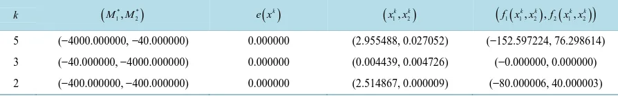
=0, x is a feasible solution. We take different parameters

(

M₁*,M₂*

)

in the MPFA algorithm, the results are shown inTable 1.

In Table 1, when M₁ or M₂ decreases, the first objective value f x x₁

(

₁, ₂

)

or f₂

(

x x₁, ₂

)

decrease too. Objective parameter can control change of each objective function. It helps decision makers learn about the change of each objective function and choose a satisfactory solution as quickly as possible.

Example 2. Consider the problem:

( )

(

1 2

) {

1 2 1 2 1 2

}

4 3 2 2 1 1 1

4 3 2 2 1 1 1 1

1 2

2 min , 2 , 2 ,

s.t. 2 8 8 2

4 32 88 96 36

0 3

0 4

P f x x x x x x x x

x x x x

x x x x x

x x = − − + − − ≤ − + + ≤ − + − + ≤ ≤ ≤ ≤

We want to find a solution that three objectives are as small as possible with the first and second objective value less than −2 and the third objective value less than −5.

Let penalty function

(

)

{

}

{

}

{

}

{

}

{

}

{

}

{

}

{

}

2

2 2

1 2 1 1 2 2 1 2 3

2 ₂

4 3 2

2 1 1 1 1

2 2 2

2 1 2

, , max 2 , 0 max 2 , 0 max , 0

max 2 8 8 2, 0 max 3, 0

max 4, 0 max , 0 max , 0 .

x x x M x x M x x M

x x x x x

x x x

ρ

ρ ρ

ρ ρ ρ

= − − + − + − + − − −

+ − + − − + −

+ − + − + −

F M

Let the starting point

(

0 0

)

( )

1, 1 0, 0

Table 1. Numerical results with different objective parameters.

k

(

* *

)

1, 2

M M

( )

k

e x

(

1, 2

)

k k

x x

(

1

(

1, 2

) (

, 2 1, 2

)

)

k k k k

f x x f x x

5 (−4000.000000, −40.000000) 0.000000 (2.955488, 0.027052) (−152.597224, 76.298614)

3 (−40.000000, −4000.000000) 0.000000 (0.004439, 0.004726) (−0.000000, 0.000000)

[image:8.595.91.538.102.172.2]

2 (−400.000000, −400.000000) 0.000000 (2.514867, 0.000009) (−80.000006, 40.000003)

Table 2. Numerical results with different objective parameters.

k

(

* * *

)

1, 2, 3

M M M

( )

k

e x

(

1, 2

)

k k

x x

(

1

(

1, 2

) (

, 2 1, 2

) (

, 3 1, 2

)

)

k k k k k k

f x x f x x f x x

5 (−10.000000, −10.000000, −10.000000) 0.000000 (2.329518, 3.178479) (−4.027439, −1.480558, −5.507997)

5 (−10.000000, −20.000000, −10.000000) 0.000000 (2.534721, 2.039602) (−1.544482, −3.029841, −4.574323)

5 (−11.000000, −20.000000, −10.000000) 0.000000 (2.489790, 2.311039) (−2.132288, −2.668541, −4.800829)

5 (−12.000000, −20.000000, −10.000000) 0.000000 (2.444095, 2.577823) (−2.711552, −2.310366, −5.021918)

( )

{

4 3 2

}

{

}

{

}

{

}

{

}

2 1 1 1 1 2 1 2

max 2 8 8 2, 0 max 3, 0 max 4, 0 max , 0 max , 0 .

e x = x − x + x − x − + x − + x − + −x + −x

We take different parameters

(

* * *

)

1, 2, 3

M M M in the MPFA algorithm and get the results shown in Table 2. In Table 2, we find a satisfactory solution

(

x x₁, ₂

) (

= 2.444095, 2.577823

)

when taking different

(

* * *

)

1, 2, 3

M M M .

4. Conclusion

In this paper, we define a penalty function with objective parameters and constraint penalty parameter for MP and the corresponding unconstraint penalty optimization problem. Under some conditions, we prove that a Pareto efficient solution (or a weakly-efficient solution) to UPOP is a Pareto efficient solution (or a weakly- efficient solution) to MP, and the penalty function is exact under a stable condition. We present the MPFA algorithm to solve the multi-objective programming with inequality constraints by using the nonlinear penalty function with objective parameters. With this algorithm, we may find a satisfactory solution.

Acknowledgments

We thank the Editor and the referee for their comments. The research is supported by the National Natural Science Foundation of China under grunt 11271329 and 10971193.

References

[1] Sawaragi, Y., Nakayama, H. and Tanino, T. (1985) Theory of Multiobjective Optimization. Academic Press, London.

[2] White. D.J. (1984) Multiobjective Programming and Penalty Functions. Journal of Optimization Theory and Applica-tions, 43, 583-599. http://dx.doi.org/10.1007/BF00935007

[3] Sunaga, T., Mazeed, M.A. and Kondo, E. (1988) A Penalty Function Formulation for Interactive Multiobjective Pro-gramming Problems. Lecture Notes in Control and Information Sciences, 113, 221-230.

http://dx.doi.org/10.1007/BFb0042790

[4] Ruan, G.Z. and Huang, X.X. (1992) Weak Calmness and Weak Stability of Multiobjective Programming and Exact Penalty Functions. Journal of Mathematics and System Science, 12, 148-157.

[5] Liu. J.C. (1996)

ε

-Pareto Optimality for Nondifferentiable Multiobjective Programming via Penalty Function. Jour-nal of Mathematical AJour-nalysis and Applications, 198, 248-261. http://dx.doi.org/10.1006/jmaa.1996.0080

[6] Huang, X.X. and Yang, X.Q. (2002) Nonlinear Lagrangian for Multiobjective Optimization to Duality and Exact Pena-lization. SIAM Journal on Optimization, 13, 675-692. http://dx.doi.org/10.1137/S1052623401384850

Operational Research, 199, 9-20. http://dx.doi.org/10.1016/j.ejor.2008.10.009

[8] Antczak, T. (2012) The Vector Exact l1 Penalty Method for Nondifferentiable Convex Multiobjective Programming Problems. Applied Mathematics and Computation, 218, 9095-9106. http://dx.doi.org/10.1016/j.amc.2012.02.056 [9] Huang, X.X., Teo, K.L. and Yang, X.Q. (2006) Calmness and Exact Penalization in Vector Optimization with Cone

Constraints. Computational Optimization and Applications, 35, 47-67. http://dx.doi.org/10.1007/s10589-006-6441-5 [10] Huang, X.X. (2012) Calmness and Exact Penalization in Constrained Scalar Set-Valued Optimization. Journal of

Op-timization Theory and Applications, 154, 108-119. http://dx.doi.org/10.1007/s10957-012-9998-4

[11] Meng, Z.Q., Shen, R. and Jiang, M. (2011) An Objective Penalty Functions Algorithm for Multiobjective Optimization Problem. American Journal of Operations Research, 1, 229-235. http://dx.doi.org/10.4236/ajor.2011.14026

[12] Luque, M., Ruiz, F. and Steuer, R.E. (2010) Modi-Fied Interactive Chebyshev Algorithm (MICA) for Convex Mul-tiobjective Programming. European Journal of Op-Erational Research, 204, 557-564.