Application of Hierarchical Linear Models/Linear
Mixed-effects Models in School Effectiveness Research
H. W. Ker
Department of International Trade, Chihlee Institute of Technology, Wunhua Rd., Banciao District, New Taipei City, Taiwan *Corresponding Author: [email protected]
Copyright © 2014 Horizon Research Publishing All rights reserved.
Abstract
Multilevel data are very common in educational research. Hierarchical linear models/linear mixed-effects models (HLMs/LMEs) are often utilized to analyze multilevel data nowadays. This paper discusses the problems of utilizing ordinary regressions for modeling multilevel educational data, compare the data analytic results from three regression techniques, and demonstrate the appropriate use of HLMs/LMEs in school effectiveness research. An analysis of a subset of NELS-88 data in which students are nested within schools is used to illustrate features of HLMs/LMEs, relative to both student-level analysis that ignores the hierarchy of the dataset, and school-level analysis that aggregate the student-level units. The features and advantages of HLMs/LMEs in multilevel educational data analysis are discussed. Some guidelines, caveats, suggestions and recommendations in utilizing HLMs/LMEs for analyzing multilevel educational data are highlighted.Keywords
Linear Mixed-Effects Models, Hierarchical Linear Models, Random Effects, Fixed Effects, Multilevel Educational Data1. Introduction
Hierarchical data structures are very common in educational research. For example, schooling systems are an example of a hierarchical structure, with students nested within classrooms, grade levels, schools, and school districts. The main goal of ‘school effectiveness’ research is to describe the differences within and between schools. For example, an investigator may want to know to what extent of differences in average exam results between schools are accounted for by factors such as intake achievements of students, students’ social-economic status (SES), characteristics of students, average class sizes, school types (public or private), and regions of school. In this case, students are level-1 units and schools are level-2 units. Level-1 predictors are intake achievements of students, students’ SES, and characteristics of students. Level-2
predictors are average class sizes, school types, and regions of school. Data that repeatedly collected on an individual student is another type of hierarchical data in a sense that the repeated measures are nested within individuals [1] [2]. For example, a researcher may want to investigate that keeping gifted students in the ordinary class or separate class will lead to better performance. The researcher may have the measures from several achievement scores during the time segment of investigation, and the score of aptitude test available. The repeated measures of performance can be viewed as level-1 units which are in terms of nested within the individual student.
The existence of data hierarchies is not ignorable [3]. Hierarchical data do present several problems for traditional data analytic techniques such as ordinary regressions. These problems are discussed as follows:
invalid results and come to wrong conclusions for studying the casual relationships.
2. Problem of the ways to deal with cross-level data: In educational research, it is often the case that a researcher is interested in investigating the relationships between environmental factors (e.g., teaching styles, teacher behaviors, class sizes, educational policies, etc.) and individual outcomes (e.g., performance, attitudes, behaviors, etc.). But given that outcomes are collected at the student level, and other variables at group levels (e.g., classroom, schools, school districts), the question arises as how to deal with cross-level interaction. One approach is to bring group-level variables down to student level (i.e., assign classrooms, teachers, or school characteristics to all students). This results in two problems. The first is that the resulting statistical inferences (i.e., significance tests) are biased and typically over-optimistic [5]. The second is that failure to incorporate schools in the statistical model means that the influence of school is ignorable [6]. The other way to deal with the problem of cross-level data is to aggregate student levels up to group levels which means that do regression over the means of group level. This aggregated analysis has several problems. The first is that much of the individual variability on outcome variable is lost. It can lead to under- or over-estimation of observed relationships between variables [7]. The second is that outcome variable change significantly and substantively from individual achievement to average group-level achievement. Furthermore, disregarding within-school variance will yield a large increase of multiple correlation coefficients [6]. Neither disaggregated analyses nor aggregated analyses can adequately describe the nature of hierarchical data well. What are required are models which simultaneously can model student level relationships and take into account of grouping. 3. The problem of the units of analysis: A classic and
well-known example on the units of analysis is a study on the ways of teaching reading for elementary school students carried out by Bennett [8]. The results showed that there exist statistically significant differences between ways of teaching (i.e., so-called ‘formal’ style of teaching reading is better than other methods). The data were using multiple regressions where students are the units of analysis. However, Aitkin & Hinde [9] reanalyzed the data and showed that when the grouping of students into class was taken account, the significant differences disappeared. This reanalysis is the important example of a multilevel analysis of educational data, using information from both “higher” level units and “lower” level units.
Hierarchical linear models/linear mixed-effects models (HLMs/LMEs) have received a lot of attention in many fields because of their flexibility in analyzing hierarchical
data. They are the extension of linear models. The application of multilevel analysis for educational hierarchical data has several advantages. First, it enables the researchers to obtain statistically efficient estimates of regression coefficients. Secondly, by using the grouping information, it provides correct standard errors, confidence intervals and significant tests [10]. Only appropriate statistical analysis can provide valid results. Thirdly, by specifying patterned variance- covariance matrices, it can help to describe the complexities of variation among higher level, especially when the covariance models are of research interest. Fourthly, by allowing the use of covariates or predictors measured at any levels of hierarchy, it enables researcher to explore the cross-level interaction. Fifthly, HLMs/LMEs can solve the confounding problem from different levels by decomposing the variables into the components according to the levels of variables [11]. In a student-school hierarchical structure, for example, the average social and economic status (SES) of a school may have influence on students’ learning on the effects of an individual student’s SES. SES at school level may represent the source of school effectiveness. SES at student level is a measure of the resource of individual home environment and family support. The variable SES at different levels has different meanings. HLMs/LMEs solve the confounding problem of variables by specifying the variables at appropriate levels, i.e., student’s SES is put in level-1 model and school average SES is specifying in level-2 model.
Researchers has to take data structure into account in data analysis because ignoring the hierarchical data structure would invalidate most traditional statistical analysis methods (i.e., independent observation), and risk overlooking important group effects and within group dependencies. The goals of this paper are to discuss the problems of employing ordinary regression in analyzing multilevel data and how it should be dealt with appropriately, and to provide examples to compare the three regression techniques (disaggregated analysis, aggregated analysis, and HLMs/LMEs) and demonstrate doing appropriate analyses. An analysis of a subset of NELS-88 data in which students are nested within schools is used to illustrate features of HLMs/LMEs, relative to both student-level analysis that ignores the hierarchy of the dataset, and school-level analysis that aggregate the student-level units. The features and advantages of HLMs/LMEs in multilevel data analysis are discussed. Several precautions and recommendations on the applications of HLMs/LMEs are suggested. This paper is mainly conceptual oriented. It does not contain the very detailed technical aspects and procedures needed to implement multilevel analysis. The readers interested in HLMs/LMEs are encouraged to refer to other suggested multilevel readings [12] [13], [26] [14] [6] [15] [2] [5] [16] for a full description of the methodological detail of HLMs/LMEs.
HLMs/LMEs are indispensable tools for analyzing hierarchically structured data in psychological, educational, medical, organizational, geographic, social behavioral, and child growth research [17] [12] [18]. For examples, Francis, Fletcher, Stuebing, Davidson, and Thompson [19] applied individual growth curves approach to the analysis of change of recovery of cognitive function following pediatric closed head injury. Kreft and Yoon [20] addressed the advantages of HLMs/LMEs for studying school effectiveness research. Huttenlocher, Haight, Bryk, Seltzer, and Lyons [23] applied HLM in studying early vocabulary growth. Barnett, Raudenbush, Brennan, and Pleck [22] utilized HLM in a longitudinal study regarding job change, marital experiences and change in psychological distress. Kidwell, Mossholder, and Bennet [23] studied the contextual effects on organizational citizenship behavior.
HLMs/LMEs are known as “hierarchical linear models”, “multilevel models” [12], “random coefficient models,” or “linear mixed-effects models” [24]. The term “hierarchical linear models” or “multilevel models” captures the characteristics of the model. The models are separated into levels. The models are appropriate for data that are hierarchically structured with lower-level units nested within higher-level units. [25]. The intercept and slopes at lower-level model become the outcomes of higher-level model. The term “random coefficient models” or “linear mixed-effects models” can be explained from experimental designs and the distributions of parameters in regression form. Random coefficient models include the parameters (i.e., intercepts, slopes) that describe the distributions of the variances of group-level statistics (i.e., group intercepts or group slopes). Therefore, they are so-called “random effects” or “random coefficients.” In experimental research, the random effects describe the levels of treatments that are assumed be sampled from a population and inferences refer to this population [24]. Random coefficient models can also describe a type of linear or nonlinear forms where the parameters are assumed to vary from a certain probability distribution.[29]. Linear mixed-effects models are mixed-effects models in which both fixed and random effects occur linearly in the model function [27].
HLMs/LMEs allow researchers to analyze hierarchically nested data with two or more levels. For example, a student-school hierarchical linear model consists of two submodels: student-level (level-1) and school-level (level-2). The parameters in a school-level model specify the unknown distribution of student-level parameters. The intercept and slopes at student-level can be specified as random. Substituting the level-2 equations for the slopes and intercepts into the level-1 model yields a linear mixed-effects model. Researchers can specify the effects of level-1 coefficients depending on their research interest or the empirical evidence shown in data.
HLMs/LMEs have the advantages of allowing researchers to specify the individual-level parameters as randomly varying across groups. It provides a compromise between modeling each group by a separate individual regression
model, and modeling all groups simultaneously by using a single regression equation [29]. Three common methods for estimating the parameters in HLMs/LMEs are maximum likelihood estimation (MLE), restricted maximum likelihood (REML) and Bayes estimation [31] [32].
A number of estimation algorithms have been derived to implement the methods of estimation. Raudenbush [32] did an intensive review on these algorithms. Aitkin and Longford [33], and Longford [24][34] developed a Fisher scoring algorithm for the maximum likelihood estimation of covariance components in multilevel mixed linear models. Goldstein[35] used iterative generalized least squares approach to obtain maximum likelihood estimate of multilevel mixed linear models. Lindley and Smith[31] derived Bayesian estimates for hierarchical linear model. Dempster, Laird, and Rubin[36] established that EM algorithm numerically obtained maximum likelihood estimates, a result with special relevance for covariance component estimation. The common algorithms that implement these estimation methods are iterative generalized least square, Fisher scoring and expectation-maximization.
There is still controversy about which estimation method with which algorithm should be used under particular sampling conditions. When the number of the units in group-level is large, any estimation method can be employed. However, parameter estimation is more problematic when the number of the units in group-level is small, because the group-level regression coefficients and individual effects are conditional upon the estimated values of group-level variance, and the variance might be underestimated [26] [37].
Bayesian estimation is usually used in simple HLMs/LMEs because the numerical integration for complex models is computationally intensive and are not easy to program. However, when the sample size is large, MLE and REML approaches work well and the Bayesian approach is not necessary [11].
In a two-level hierarchical model, the MLE and REML approaches produce very similar results for
σ
2, but there are some differences in estimating the level-2 variance-covariance components. MLE and REML approaches have very similar results if the number of level-2 units (J) is large. On the other hand, if the number of level-2 units is small, the MLE variance estimates are smaller than the REML estimates. REML minimizes least squares residuals and is generally considered better than the maximum likelihood method based on the deviance of the data only. However, de Leeuw and Kreft [38](1995, p.183) noted that “ the evidence of their superiority in complicated cases, and in multilevel analysis in particular, is not too convincing.”superiority in complicated models is still in question [38]. Bayes estimation does not have the restrictions that MLE and REML have; however, Bayesian estimation may not be feasible for complicated models due to the computational demands of multiple numerical integration requirements [7].
Anderson [39] summarized the comparison between REML and MLE as follows:
1. Both estimation methods are based on the maximum likelihood principles and the estimators from MLE and REML are consistent, efficient and asymptotically normal.
2. MLE provides the estimates for fixed effects whereas REML does not.
3. With the univariate normal population and standard linear regression models, the estimated means are the same under MLE and REML. However, the vector of fixed effects is not the same under MLE and REML in linear mixed-effects models.
4. In a balanced design, REML estimators yields the same results as obtained from classical ANOVA-type estimates.
5. The estimated variance components are larger in REML than in ML.
6. ML and REML estimations differ more when the number of parameters in fixed effects increases. 7. Likelihood ratio tests on variance components can be
used with models fit by REML or MLE. Both models must be fit by REML and the fixed-effects structures must be the same for both models.
8. Likelihood ratio tests for fixed effects can be used only for MLE. They aren’t valid for REML.
3. Example
3.1. The Data Set
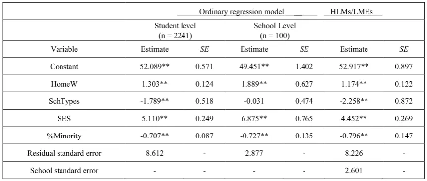
For the illustration of the three statistical strategies (disaggregation, aggregation, and HLMs/LMEs) for analyzing multilevel educational data, a subset of the National Educational Longitudinal Survey of 1988 (NELS-88) data was used. The data were collected by the National Center for Education Statistics of the US Department of Education. The data contains a representative sample of approximately 1000 schools across United States that enroll more than 20,000 eighth graders in the base year study. The data are at a variety of levels, including individual students, family, teachers, and schools [6] [4]. In this analysis, 100 out of 1003 schools were randomly selected. There are 2241 students in this subset. The outcome variable is math achievement (Math). The explanatory variables are student socioeconomic status (SES), the number of hours of homework (HomeW), the school types (SchTypes, public schools are coded 1 and private schools coded 0), and the percent of students in the schools who are members of racial minority groups (%Minority). SES and HomeW are level-1 predictors, and SchTypes and %Minority are level-2 variables. In general, SES and HomeW are expected positively related to math achievement, and SchTypes and %Minority are negatively related to math achievement. Three regression models (disaggration, aggregation, and HLMs/LMEs) were fit to this subset of NELS-88 data. Results from these analyses are given in Table 1. The first two columns of Table 1 give results of ordinary regression models at student level and school level, and the third column gives the results from HLMs/LMEs. The estimation method for HLMs/LMEs is REML.
[image:4.595.89.520.510.693.2]3.2. A Comparison of Regression Models
Table 1. Comparison of Three Regression Models for a Subset of NELS-88 Data
Ordinary regression model __ HLMs/LMEs Student level
(n = 2241) School Level (n = 100)
Variable Estimate SE Estimate SE Estimate SE
Constant 52.089** 0.571 49.451** 1.402 52.917** 0.897
HomeW 1.303** 0.124 1.889** 0.627 1.174** 0.122
SchTypes -1.789** 0.518 -0.031 0.474 -2.258** 0.872
SES 5.110** 0.249 6.875** 0.765 4.452** 0.269
%Minority -0.707** 0.087 -0.727** 0.135 -0.796** 0.147
Residual standard error 8.612 - 2.877 - 8.226 -
School standard error - - - - 2.601 -
Disaggregated analysis. The student level analysis ignored the hierarchical structure that students are nested within schools and treated as independent observations. It also means that no systematic influence of the schools on math achievement is expected, and all influence of the school are in residual errors. The resulting model was significant, with R-squared = 0.308, F (4, 2236) = 248.5, p < .0001. All four predictors were significant predictors of students’ math achievement. As expected, SES and HomeW are expected positively related to math achievement, and SchTypes and %Minority are negatively related to math achievement.
Aggregated analysis. In school-level analysis, all student-level variables were aggregated up to school level by averaging. This strategy ignores all within-school variation and cannot make any inferences or predictions directly for individual students. The resulting model was significant, with R-squared = 0.752, F (4, 95) = 72.150, p < .0001. Both average SES and average HomeW were significantly positively related to math achievement. The predictor %Minority was negatively related to math achievement. In this analysis, SchTypes was not a significant predictor of average math achievements.
Multilevel analysis. A random intercept model was performed via HLM, in which the respective level 1 and level 2 predictors were specified appropriately. In multilevel analysis, the variance for outcome variable is broken into level-1 and level-2 variance. The residual standard error between schools is 2.601, and the residual standard error between students is 8.226. The absolute value of log-likelihood is 7959.898. The intraclass correlation is 0.24 (2.601/(8.226+2.601) ), indicating that about 24% of the variance in math achievement is between schools. This analysis shows that significant positive effects of level-1 predictors on math achievement, and negative relationships between math achievement and level-2 predictors.
4. Discussion on the Three Regression
Models
The example above demonstrates that the selection of statistical models can influence the conclusions drawn from a given data set. In comparison, the multilevel model is assumed that it represents the best estimate of the true relationships between the predictors and the outcome. Compared with disaggregated analysis, the aggregated analysis overestimated the value of R-squared 144%. Compared with HLMs/LMEs, the aggregated analysis overestimated the regression coefficients of level-1 predictors, while underestimated the regression coefficients of level-2 predictors. For example, it overestimated the regression coefficient for HomeW by 61% and SES by 54%, and underestimated the slope for SchTypes by 98% and for %Minority by 9%. Using aggregated analysis at the
school level only produce a nonsignificant SchTypes. The results from aggregated analysis evidence the previous discussion: the aggregated analysis yield a large increase of multiple correlation coefficient, and under- or over-estimate the regression coefficients.
The standard error of intercept is approximately twice as large in the results from random intercept model as in that from the disaggrated analysis. This implies that the disaggregate analysis produces an over-optimistic impression of the precision of this estimate, and illustrate the risk of overlooking the hierarchical structure in data analysis. Generally the standard errors from disaggregated model are smaller than those from multilevel models. The residual error is higher in the disaggregated model because the multilevel model allows for additional parameter to model the variation. The values of the regression coefficients at level-1 predictors (HomeW and SES) in the disaggregated and multilevel model are very close. This is because in REML, the fixed-effects coefficients are estimated with least squares methods as well. However, the relationships between outcome and level-2 predictors (SchTypes and %Minority) are stronger in the multilevel model than those in disaggregated models. The standard errors at level-2 predictors are larger in multilevel model than in disaggregated model because single-level analysis tends to produce biased standard errors (generally lower than they should be) for the coefficients defined at level 2.
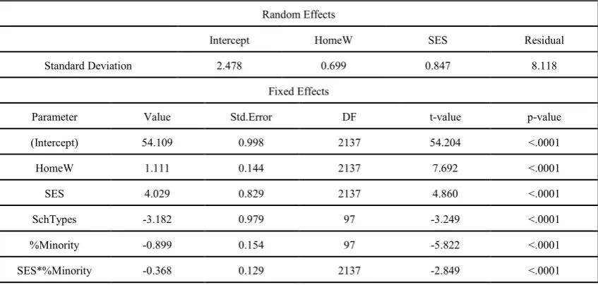
This subset of NELS-88 can be further analyzed to investigate the possible cross-level interaction effects. A random intercepts and slopes model is fit to the data with the level-1 intercept and slopes (HomeW and SES) having SchTypes and %Minority as predictors. After standard HLMs/LMEs model-building procedure and model reduction, Table 2 is the results for the random intercepts and slopes model.
Table 2. Results of Multilevel Models with Cross-level Interaction
Random Effects
Intercept HomeW SES Residual
Standard Deviation 2.478 0.699 0.847 8.118
Fixed Effects
Parameter Value Std.Error DF t-value p-value
(Intercept) 54.109 0.998 2137 54.204 <.0001
HomeW 1.111 0.144 2137 7.692 <.0001
SES 4.029 0.829 2137 4.860 <.0001
SchTypes -3.182 0.979 97 -3.249 <.0001
%Minority -0.899 0.154 97 -5.822 <.0001
SES*%Minority -0.368 0.129 2137 -2.849 <.0001
Note. (a) Model fit: AIC=15923.44, BIC=16003.44, logLik=-7947.72
5. Conclusions and Suggestions
The example demonstrated above highlight the features of multilevel models for analyzing educational data and how analysis by traditional regression models at single level can lead to biased estimated of standard errors and draw different conclusion. As demonstrated, HLMs/LMEs provide a powerful tool for analysis of hierarchical data. Alternatively, traditional analysis at the individual level or group level is problematic. Traditional analysis at individual level ignores dependence in the data that results from grouping, whereas analysis at the group level does not permit a straightforward inferences or prediction for individual. Traditional analysis cannot accurately model the true relationship between outcome and predictors. HLMs/ LMEs can include independent variables at either group or individual level and estimate their effects as well as interactions. The advantages of multilevel modeling include producing statistically efficient estimates of regression coefficients, correct standard errors, confidence intervals, and significant tests, can use covariates measured at any levels of hierarchy. With hierarchical data common in educational research, and with recent advanced developments of statistical software for the ease of performing multilevel modeling, it is hoped that educational researchers can become more acquainted with the procedures and rational of HLMs/LMES in analyzing hierarchical data.
Although HLMs/ LMEs have many advantages in analyzing hierarchical data, they are not necessary in some circumstances. It should be noted that multilevel modeling approach can not be applied blindly. Researchers should be able to judge the circumstances where HLMs/LMEs are appropriate in analyzing hierarchical data. In some cases, separate regression line for each group is more appropriate. For example it is appropriate to fit separate regression line for each school if only a few schools involved and each with a large number of students, or researchers only want to make
inferences about those specific schools. However, if these schools are regarded as a random sample from a population of schools and the research interest is to make inferences about the variation between schools in general, then a multilevel approach necessary. In some cases, standard multiple regressions and other single-level statistical methods are more appropriate. HLMs/LMEs are useful when random factors are present in multilevel data. When data do not show between-subjects variability, the cases have very large groups with very small intra-class correlations, the data already provide all information needed and inference only apply to the specified groups, or the research interest is to compare the average performance among groups, HLMs/LMEs are not necessary. In these cases, standard multiple regression methods, dummy variable regression, or varied experimental design techniques are enough to analyze data. Moreover, it should be careful in specifying the effects of the parameters in building HLMs/LMEs. Fixing an effect can change the results of the significant test on that effect as well as the estimates of other parameters. General guidelines to specify a fixed or random effect cannot apply to all situations. Models with too many parameters specified as random effects may have difficulty in convergence. Hence it is crucial to carefully examine the data structure, the results, and the underlying theory of the study before specifying fixed or random effects.
to show the need of utilizing HLMs/LMEs (i.e., data have between-subjects variability) as well as the nature and the patterns of data structure. In model-building process, graphical methods should be able to guide the forms of fixed effects, the variance-covariance models, and the models for within-subject errors. In model-checking, it should help to understand the numerical facts for the results from the tests of assumptions. In other words, the questions often addressed in multilevel research—including characterizing or describing the patterns at both the group and individual levels, identifying the important predictors and unusual subjects, choosing suitable statistical models, selecting random-effects structures, suggesting possible residuals covariance models, and examining the model-fits—can be answered via visual-graphical methods. Conventional visualization methods, new graphical techniques, and the advance of graphical technology in computational ability should be integrated into a systematic procedure to suit multilevel modeling.
Multilevel data are very common in social science research, especially challenging in educational field. HLMs/LMEs are often utilized to analyze multilevel data nowadays. This paper discusses the problems of utilizing ordinary regressions in analyzing multilevel educational data, compares three data analytic results from regression techniques, and demonstrates the appropriate uses of HLMs/LMEs. Some caveats and recommendations in utilizing HLMs/LMEs are highlighted. The attempt here is to advocate HLMs/LMEs as an alternative in analyzing multilevel educational data as well as provide guidelines and suggestions in appropriate use of multilevel modeling.
REFERENCES
[1] E. F.Vonesh, & V. M. Chinchilli, (1997). Linear and nonlinear models for the analysis of repeated measurements. New York: Marcel Dekker, Inc.
[2] J.D. Singer, & J.B. Willett, (2003). Applied Longitudinal Data Analysis: Modeling Change and Event Occurrence. NY: Oxford University Press.
[3] H. Goldstein, (1997). Methods in school effectiveness research. School Effectiveness and School Improvement,8, 369-395.
[4] C. J. Osborne, (2000). Advantages of hierarchical linear modeling. Practical Assessment, Research & Evaluation, 7 (1). Retrieved October 30, 2001, from http://PAREonline.net [5] T. Snijders, & R. Bosker, (1999). Multilevel analysis: An
introduction to basic and advanced multilevel modeling. CA: Sage.
[6] I. Kreft, & J. de Leeuw, (1998). Introducing multilevel modeling. Thousand Oaks: Sage.
[7] A.S. Bryk, & S.W. Raudenbush, (1992). Hierarchical linear models: Applications and data analysis methods. CA: Sage.
[8] N. Bennett, (1976). Teaching styles and pupil progress. London: Open Books.
[9] M. Aitkin, , & J. Hinde, (1981). Statistical modeling of data on teaching style. Journal of the Royal Statistical Society, A, 144, 419-461.
[10] C. J. Anderson, (2004a). Introduction to hierarchical linear models. (2003, Oct 29). Retrieved August 10, 2004, from http://www.ed.uiuc.edu/courses/edpsy490ck
[11] S. W. Raudenbush, & A. S. Bryk, (2002). Hierarchical linear models: Applications and data analysis methods. CA: Sage. [12] H. Goldstein, (1995). Multilevel statistical model (2nd ed.).
New York: Halsted.
[13] H. Goldstein, (1999). Multilevel statistical models, Internet version. (http://www.ioe.ac.uk/multilevel).
[14] J.J. Hox, (2002). Multilevel Analysis: Techniques and Applications. Mahwah: N.J.: Earlbaum
[15] D.A. Luke, (2004). Multilevel Modeling. Thousand Oaks: Sage Publications.
[16] G. Verbeke, & G. Moldenberghs, (2000). Linear mixed models for longitudinal data. NY: Springer-Verlag.
[17] D. Draper, (1995). Inference and hierarchical modeling in the social science. Journal of Educaational and Behavioral Statistics, 20, 115-147.
[18] B. N. Pollack, (1998). Hierarchical linear modeling and the “unit of analysis” problem: A solution for analyzing responses of intact group member. Group Dynamics: Theory, Research, and Practice, 2, 299-312
[19] D. J.Francis, J. M. Fletcher, K. K. Stuebing, K. C.Davidson, & N. M. Thompson, (1991). Analysis of change: Modeling individual growth. Journal of Counseling and Clinical Psychology, 59, 27-37.
[20] G. G. Kreft, & B. Yoon, (1994). Are multilevel techniques necessary? An attempt at demystification. ERIC document, ED371033.
[21] J. Huttenlocher, W. Haight, A. Bryk, M. Seltzer , & T. Lyons, (1991). Early vocabulary growth: Relation to language input and gender. Developmental Psychology, 27, 236-248. [22] R. C.Barnett, S. W. Raudenbush, R. T. Brennan, & J. H.
Pleck, (1995). Change in job and martial experience and change in psychological distress: A longitudinal study of dual-earner couples. Journal of Personality and Social Psychology, 69, 839-850.
[23] R. E. Kidwell, Jr., K. M. Mossholder, & N. Bennet, (1997). Cohesiveness and organizational citizenship behavior: A multilevel analysis using work groups and individuals. Journal of Management, 23, 775-793.
[24] N. T. Longford, (1993). Random coefficient models. New York: Oxford University Press.
[25] S.W. Raudenbush, (1993). Hierarchical linear models and experimental design. In L. Edwards (Ed.), Applied analysis of variance in behavioral science. New York: Marcel Dekker, 459-496.
Associate.
[27] J. C. Pinherio, & D. M. Bates, (2000). Mixed-effects models in S and S-Plus. New York: Springer-Verlag.
[28] J. J. Hox, (2000). Multilevel analysis of grouped and psychological longitudinal data. In T. D. Little, K. U. Schnabel, & J. Baumert (Ed.), Modeling longitudinal and multilevel data: Practical issues, applied approaches and specific examples (pp. 15-32). NJ: Lawrence Erlbaum Associates.
[29] R. C. MacCallum, & C. Kim, (2000). Modeling multivariate change. In T. D. Little, K. U. Schnabel, & J. Baumert (Ed.), Modeling longitudinal and multilevel data: Practical issues, applied approaches and specific examples (pp. 51-68). NJ: Lawrence Erlbaum Associates.
[30] D. Hedeker, (2004). Mixed models for longitudinal data: An applied introduction. (n.d.). Retrived May 16, 2004, from http://www.uic.edu/~hedeker/long.html.
[31] D. V. Lindley, & A. F. M. Smith, (1972). Bayes estimates for the linear model. Journal of the Royal Statistical Society, Series B, 34, 1-41.
[32] S. W. Raudenbush, (1988). Educational application of
hierarchical linear model: A review. Journal of Educational Statistics, 13, 85-116.
[33] M. Aitkin, , & N. T. Longford, (1986). Statistical modeling issues in school effectiveness studies. Journal of the Royal Statistical Society, Series A, 149, 1-43.
[34] N. T. Longford, (1995). Random coefficient models. In G. Arminger, C. C. Clogg, & M. E. Sobel (Ed), Handbook of statistical modeling for the social and behavioral science (pp. 519-577). New York: Plenum Press
[35] H. Goldstein, (1986). Multilevel linear mixed model analysis using iterative generalized least square. Biometrika, 73(1), 43-56.
[36] A. P. Dempster, N. M. Laird, & D. B. Rubin, (1977). Maximum likelihood for incomplete data via the EM algorithm. Journal of the Royal Statistical Society, Series B, 39, 1-18.
[37] C. Morris, (1995). Hierarchical models for educational data: An overview. Journal of Educational Statistics, 20, 190-200 [38] J. de Leeuw, & I. G. Kreft, (1995). Questioning multilevel