LEABHARLANN CHOLAISTE NA TRIONOIDE, BAILE ATHA CLIATH TRINITY COLLEGE LIBRARY DUBLIN OUscoil Atha Cliath The University of Dublin
Terms and Conditions of Use of Digitised Theses from Trinity College Library Dublin
Copyright statement
All material supplied by Trinity College Library is protected by copyright (under the Copyright and Related Rights Act, 2000 as amended) and other relevant Intellectual Property Rights. By accessing and using a Digitised Thesis from Trinity College Library you acknowledge that all Intellectual Property Rights in any Works supplied are the sole and exclusive property of the copyright and/or other I PR holder. Specific copyright holders may not be explicitly identified. Use of materials from other sources within a thesis should not be construed as a claim over them.
A non-exclusive, non-transferable licence is hereby granted to those using or reproducing, in whole or in part, the material for valid purposes, providing the copyright owners are acknowledged using the normal conventions. Where specific permission to use material is required, this is identified and such permission must be sought from the copyright holder or agency cited.
Liability statement
By using a Digitised Thesis, I accept that Trinity College Dublin bears no legal responsibility for the accuracy, legality or comprehensiveness of materials contained within the thesis, and that Trinity College Dublin accepts no liability for indirect, consequential, or incidental, damages or losses arising from use of the thesis for whatever reason. Information located in a thesis may be subject to specific use constraints, details of which may not be explicitly described. It is the responsibility of potential and actual users to be aware of such constraints and to abide by them. By making use of material from a digitised thesis, you accept these copyright and disclaimer provisions. Where it is brought to the attention of Trinity College Library that there may be a breach of copyright or other restraint, it is the policy to withdraw or take down access to a thesis while the issue is being resolved.
Access Agreement
By using a Digitised Thesis from Trinity College Library you are bound by the following Terms & Conditions. Please read them carefully.
S tatistical M odels For Food
A u th en ticity
A thesis subm itted to th e University of D ubhn, Trinity College
in p artial fulfillment of th e requirem ents for th e degree of
D octor in Philosophy
D epartm ent of S tatistics, University of D ublin, Trinity College
2009
T r in it y COLLEGE 2 8 JUL 2011
D ecla ra tio n
T his thesis has no t been su b m itted as an exercise for a degree a t any other University.
Except where otherw ise stated , the work described herein has been carried out by
th e au th o r alone. This thesis may be borrowed or copied upon request with the
perm ission of the Librarian, University of D ubhn, T rinity College. T he copyright
belongs jo in tly to th e University of D ublin and D eirdre A nn Toher.
A b stra ct
T he au th en tic atio n of food samples pose a particu lar problem for regulators. The routine te stin g of prem ium food products, m ost likely to be subject to m anipulation for com m ercial gain, is only feasible if the testing m ethod does not dam age the product. N ear Infrared (NIR) spectroscopy is one such m ethod th a t is b o th fast and non-invasive. However, unlike other spectroscopic m ethods, peaks in th e resulting NIR curves are a t im precise locations, requiring further statistical analysis if it is to be used for th e classification of samples.
T h ree N IR d atase ts are exam ined in this thesis two are related to the identi fication of a d u lterated samples, th e th ird is a stu d y on th e identification of types of m eats. O th er conunonly available, non-NIR, d atase ts are used for illustrative purposes.
T h e m odels developed in this thesis m ust be suitable for use by chemists with access only to personal com puters and have reasonable com putational time if they are to be ado pted into practice. Some of th e m ethods developed are refinements to existing m ethods such as the development of th e use of inform ation criteria for the selection of the num ber of param eters to use w ith P artial Least Squares Re gression and th e incorporation of a semi-supervised framework w ith F isher’s Linear D iscrim inant Analysis. A variety of dim ension reduction approaches are used with m odel-based discrim inant analysis and w ith classification based on a homogeneous group versus a heterogeneous group.
A ck n ow led gem en ts
I have been in the unusual, but fortunate position of having not one but two su pervisors for the duration of my thesis. Dr Brendan Murphy has provided me with support from a statistical viewpoint, while Dr Gerard Downey provided me with the support from a food scientist’s viewpoint. Brendan has supported my interest in statistical research from an undergraduate level and has given me all the sup port th a t could be wished for. Gerry has provided a fresh eye on my work, giving practical advice on what is needed for methods to be used by spectroscopists.
My research has been funded by the Walsh Fellowship scheme in Teagasc and the additional funding by Science Foundation Ireland has enabled me to travel to conferences and working groups both in Ireland and abroad.
I m ust thank the entire of the Statistics Department of Trinity College Dublin, especially those who contributed to the working group meetings. The feedback given at these meetings proved invaluable towards the shaping of the content of this thesis. To my fellow postgraduate students within the Department, past and present, especially those who have shared the office of room 118 - thanks for lightening the tone when required and helping me to find the appropriate words of late!
Similarly the spectroscopy group within the Ashtown Food Research Centre gave me a useful insight into the problems faced in the analysis of spectroscopy data and also into the types of problems th a t spectroscopy is considered a potentially valuable tool. The members of this group, among other postgraduate students in the Prepared Foods Department welcomed me into an unfamiliar setting of a food research facility, w ithout plaguing me too much with statistics questions over coffee.
directing my research.
My parents have managed to survive consecutive Octobers with an offspring writing their PliD thesis. Their continuing patience and support has been duly noted and greatly appreciated; my mother in particular has spent hours proofreading a thesis with no prior knowledge of chemistry or statistics. My brother Cormac too has contributed from Germany to the proofreading process, he has also provided a useful sounding board throughout rriy studies.
D eirdre A nn T oher
C on ten ts
A b stra ct i
A ck n o w led g em en ts iii
List o f T ables ix
List o f F igures xi
C h ap ter 1 In tro d u ctio n 1
1.1 M o tiv a tio n ... 1
1.2 Food Authenticity S t u d i e s ... 2
1.3 Overview of C h a p te rs ... 3
1.4 Research C o n trib u tio n s... 4
C hap ter 2 Food A u th en ticity D a ta 7 2.1 Near Infrared Spectroscopy... 7
2.1.1 Structure of NIR s p e c tru m ... 10
2.2 NIR D a t a ... 11
2.2.1 Honey S a m p le s ... 11
2.2.2 Meat S a m p le s ... 13
2.2.3 Adulterated Olive O i l s ... 15
2.3 Other Food Authenticity D a t a ... 16
2.3.1 Geographic Origin of Olive Oil S am p les... 16
2.3.2 W in e ... 17
3.1.1 A lgorithm for P L S R ... 19
3.1.2 N um ber of P a r a m e t e r s ... 20
3.2 Soft Independent M odelling of Class A n a lo g ie s... 21
3.3 Likelihood Based S tatistical In fe re n c e ... 24
3.4 M odel-based D iscrim inant A n a l y s i s ... 26
3.4.1 U pdating ... 28
3.4.2 Im plem enting the EM A l g o r i t h m ... 30
3.5 Dimension R eduction T e c h n iq u e s ... 32
3.5.1 Wavelet A n a l y s i s ... 32
3.5.2 W avelength Selection M e th o d s ... 34
3.6 Model Selection Techniques ... 36
3.6.1 Bayesian Inform ation C riterion ( B I C ) ...37
3.6.2 F fold cross v a l i d a t i o n ... 37
3.6.3 B rier’s S c o re ... 38
3.7 Performance C o m p a ris o n ... 38
3.7.1 PLSR... 39
3.7.2 Model Based M e t h o d s ... 39
3.8 C o n c lu s io n s ... 46
C h a p te r 4 G r o u p o f I n t e r e s t b a s e d C la s s ific a tio n 49 4.1 General C oncept ... 49
4.2 Variable S e le c tio n ... 53
4.2.1 Variable Selection P r o c e d u r e ... 53
4.3 Varying th e T h r e s h o l d ... 58
4.3.1 E valuating th e Threshold D ire c tly ... 59
4.3.2 Behaviour of the Threshold ... 60
4.4 R e s u lts ... 60
4.4.1 NIR d atasets ... 60
4.5 C o n c lu s io n s ... 76
C h a p t e r 5 U p d a t i n g F i s h e r ’s L in e a r D is c r im in a n t A n a ly s is 79 5.1 Fisher’s L D A ... 79
5.1.2 P r e d i c t i o n ...81
5.1.3 U pdating ...81
5.1.4 Im plem entation of Semi-supervised F ish er’s Linear Discrimi n an t A n a l y s i s ... 82
5.2 D a t a ... 86
5.2.1 F ish er’s Iris D a t a ...86
5.2.2 W ine D a t a ... 88
5.2.3 M eats D a t a ... 91
5.2.4 Honey D a t a ... 93
5.2.5 Olive Oil D a ta ... 97
5.3 C o n c l u s i o n s ... 99
C h a p t e r 6 G e n e r a lis in g F i s h e r ’s L in e a r D is c r im in a n t A n a ly s is 103 6.1 F u rth er G e n e r a lis a tio n ...103
6.1.1 Hg = ^ = X D A D ' \ f g ... 104
6.1.2 Sg = A / ...104
6.1.3 ^ g = \ g l...105
6.1.4 Zg = X g D g A g D ' g... K)6 6.1.5 Numerical A p p ro x im a tio n s...107
6.2 C o n c lu s io n s ... 108
C h a p t e r 7 C o n c lu s io n s a n d F u r t h e r W o rk 111 7.1 C o n c l u s io n s ... I l l 7.1.1 Dimension Reduction T e c h n iq u e s ... I l l 7.1.2 Identification of A dulterated S a m p le s ... 113
7.1.3 Classification for M ultiple G r o u p s ...113
7.2 F u rth er W o r k ... 114
7.2.1 R p a c k a g e ... 114
7.2.2 Im plem entation of generalised F isher’s L D A ... 114
7.2.3 Variable S e le c tio n ...114
7.3 F inal C om m ents ...115
List o f Tables
3.1 P arain etrizatio ns of th e covariance m atrix E g ... 27 3.2 Classification Performance: PLSR on Honey D a t a ... 41 3.3 Classification Performance: W avelength Selection, MBDA on Honey
D a t a ... 42 3.4 Classification Performance: W avelength Selection, MBDA on Honey
D a t a ...43 3.5 Classification Performance: W avelength Selection, MBDA on Olive
Oil D a t a ... 44 3.6 Classification Performance: W avelength Selection, MBDA on Olive
Oil D a t a ... 45 3.7 Classification Performance: PLSR on Olive Oil D ata ... 46 4.1 Classification Performance, Honey D ata: fo{x) = 1 / V ... 63 4.2 Classification Perform ance, Honey D ata: fo{x) = 6 4
4.3 Classification Perform ance, Ohve Oil D ata: f o { x ) = 1 / V ...68 4.4 Classification Perform ance, Olive Oil D ata: f o { x ) — q k f { x \ f - i k , ^ k ) 69 4.5 C om parison of E rror Rates: direct calculation of a threshold versus
T = i ^ - P g ) / P g V... 69 4.6 C om parison of E rror R ates for r calculated d i r e c t l y ... 72 4.7 R elationship of r directly calculated to 1/K : {1 — Pg)/pgV used for
variable s e l e c t i o n ... 73 4.8 R elationship of r directly calculated to \ j V \ t directly calculated
used for variable selection ... 74 4.9 Classification Performance: W avelength Selection using \ j V MBDA
5.1 Classification Performance: Iris D a t a ...88
5.2 Classification Performance: W ine D a t a ... 89
5.3 Classification Performance: Full W ine D ata ... 89
5.4 Classification Performance: M eats D a t a ... 93
5.5 Classification Performance: Honey D ata ... 93
5.6 Classification Performance: Olive Oil D a t a ... 98
List o f Figures
2.1 Electromagnetic S p e c tru m ...
9
2.2 Visible S p e c tr u m ...
9
2.3 NIR re g io n s ... 10
2.4 Sample spectra of unmodified bacteria in MRD
... 11
2.5 Flow diagram of Adulteration Process... 14
2.6 NIR spectra of h o n e y s ... 14
2.7 NIR spectra of m e a ts ... 15
2.8 NIR spectra of olive o i l s ... 16
2.9 Map of I t a l y ... 17
3.1 Volume, Shape and Orientation of E g ...28
3.2 Means Separated by 4, 2 and 1 Standard D eviation(s)... 30
3.3 Wavelet Functions ...33
3.4 Actual and Reconstructed, Thresholded S p e c tr a ...34
3.5 Wavelengths Selected using Between and Within Group Covariances . 36
4.1 Selecting the first v a r ia b le ... 56
4.2 Selecting the second variable... 56
4.3 Selecting the third variable... 57
4.4 Selecting the fourth v a ria b le ... 58
4.5 One dimensional example of the behaviour of the th resh o ld ... 59
4.6 Behaviour of r and volum e... 60
4.7 Variables selected when
f o { x )=
^k),
NIR honey data
50%/50% s p lit... 65
4.9 Variables selected when
f o { x )=
Qkf{x\fik, ^k), NIR honey data
10%/90% sp H t... 67
4.10 Variables selected when
f o { x )=
NIR olive oil
data 50%/50% s p l i t ... 70
4.11 Variables selected when
f o { x )=
9/t/(^|/^fc) S/c), NIR olive oildata 25%/75% s p l i t ... 71
4.12 Relationship between r directly calculated and 1/K: NIR, olive oil
d ata50% /50% ... 74
5.1 Projections of the Iris D a ta s e t... 87
5.2 Coefficients of the Discriminant Functions of the Iris Dataset at 10%/90%
s p l i t ... 87
5.3 Projections of the Wine D a ta s e t... 90
5.4 Coefficients of the Discriminant Functions of the Wine Dataset at
10%/90% spU t... 91
5.5 Projections of the Minced Meat Dataset
... 92
5.6 Coefficients of the Discriminant Functions of the Meats Dataset at
50%/50% s p lit...94
5.7 Projections of the Pure and Adulterated Honey Dataset: 50%:50% split 95
5.8 Projections of the Pure and Adulterated Honey Dataset: 25%:75% spht 95
5.9 Coefficients of the Discriminant Function of the Honey Dataset at
50%/50% s p lit... 97
5.10 Coefficients of the Discriminant Function of the Olive Oil Dataset at
C hapter 1
In trod u ction
1.1
M o tiv a tio n
T he m ain purpose of this thesis is to provide statistic al m ethods for use by food scientists in th e process of food authentication. A variety of different m ethods of analysing the food sam ples are considered, w ith m ost em phasis being placed on providing statistic al techniques for Near Infrared (NIR) data.
T h e m ethods developed th ro ug ho ut this thesis, while targ eted tow ards NIR data, are also designed to be suitable to more general applications: especially situations where th ere is high dim ensional, highly correlated data.
T h e statistic al techniques developed should remove th e subjectivity from the classification process when using N IR data. Introducing a probabilistic framework for th e classification process enables consistent m easures of uncertainty about the individual classification decisions to be made.
Using R for all com putations throughout this thesis enables th e m ethods to be easily reproduced for a variety of com putation platform s.
1.2
F ood A u th e n tic ity S tu d ies
T h e m ain aim of food a u th e n tic ity stu d ie s is to d e te c t w hen foods a re n o t w h a t th e y claim to be an d th e re b y p rev e n t econom ic frau d or possible d a m a g e to h e a lth . Foods th a t are su sceptible to such fra u d are th o se w hich are expensive a n d s u b je c t to th e vagaries of w eath er d u rin g gro w th or h a rv e stin g e.g. coffee, v arious fru its, h erb s an d spices. Food fra u d c a n g e n e ra te significant am o u n ts of m o n ey {e.g. several m illion US dollars) for u n sc ru p u lo u s tra d e rs so th e risk of a d u lte ra tio n is real.
T his ty p e of fra u d n o t only applies to th e consum er m a rk e t (generally th ro u g h in ac c u ra te labelling), b u t also to th e in d u stria l in g red ien ts m a rk e t, w here food tra c e- ab ility a n d q u a lity c o n tro l are of increasing im p o rta n c e . A n a ly tic a l tech n iq u es t h a t are available to in d u s try include “w et ch e m istry ” tech n iq u es - invasive a n d d e stru ctiv e, b u t easy to in te rp re t a n d o th e r non-invasive tech n iq u es t h a t req u ire m ore in te rp re ta tio n of th e re su lts such as N ear In fra re d (N IR ) spectroscopy.
Ingredient frau d can e x te n d b eyond th e ty p ical h u m an food chain. O n th e M arch 2006, th e Food an d D ru g A d m in istra tio n (FD A ) in th e U n ite d S ta te s a n nounced th a t it h ad discovered t h a t som e p e t foods were killing c a ts a n d dogs. O n fu rth e r in v estigation, th e source of c o n ta m in a tio n was found in v eg e ta b le p ro te in s im p o rte d from C h in a a n d used n o t only in p e t food, b u t also in farm an im a l an d fish feed. A lth o u g h risk to people from e a tin g th e resultcint foods w as low, it high lighted th e need for a d e q u a te co ntrols a t all p o in ts t h a t have th e p o te n tia l to e n te r th e h um an food chain.
A n even m ore serious pro b lem has em erged recently w ith th e in creased prevalence of c o n ta m in a ted or co u n te rfe ite d d ru g s, resu ltin g in ineffective, d an g e ro u s p ro d u c ts being released on to th e m ark e t. T h is is n o t a new pro b lem th e W orld H e a lth O rg an isatio n n o te d in a 1999 re p o rt t h a t th e problem is referred to in w ritin g s d a tin g back to th e fo u rth c c n tu ry BC; D ioscoridcs in th e first c e n tu ry A D in G reece identified a d u lte ra te d d ru g s a n d advised o th ers on th e ir d e te c tio n . N ew ton e t al. (2006) o u tlin e th e scale of th e p roblem a n d som e of th e c u rre n t d e te c tio n m e th o d s used in co u n terfeit d ru g d etectio n .
con-tam ination problem became evident in the later report by S. McDonald which noted th a t about 53,000 children had been sickened by the contam inated milk products.
1.3
O v erv iew o f C h a p ters
A brief outline of the research completed follows:
C h ap ter 2: F ood A u th en tic ity D a ta
Models developed throughout this thesis are applied to food authenticity problems. Examples of how such problems arise in practical terms are given and the motivation behind the solution of these problems are addressed. The specific d ata on which the methods are applied are introduced in this chapter.
C h ap ter 3: S ta tistic a l M eth o d o lo g y
Existing statistical methods are introduced, especially those th a t have been devel oped within the chemometric literature to analyse near infrared spectroscopic data. Details of the implementation of Partial Least Squares Regression, Soft Independent Modelling of Class Analogies and Model-based discriminant analysis (with and with out updating procedures) are given and the issues of model selection and evaluation are addressed.
C h ap ter 4: G roup o f In terest B ased C lassification
C hapter 5: U p d a tin g F ish er’s Linear D iscrim in ant A n a ly sis
Finding a projection of the d ata th a t maximises the separability of groups enables the elimination of the need for separate dimension reduction. Fisher’s Linear Dis criminant Analysis is generalised to incorporate a semi supervised perspective.
C hapter 6: G en eralisin g F ish er’s Linear D iscrim in an t A n a ly sis
Fisher’s Linear Discriminant Analysis assumes th a t the covariance matrices are the same across groups. This is generalised using the likelihood ratio so th a t the restric tion that all the covariance matrices are the same can be relaxed.
C hapter 7: C on clu sion s and Further W ork
This chapter summarises the findings of the different approaches towards dimension reduction. It also compares the relative appropriateness of the different discrimi nation approaches for both two group and multiple group classification problems. Areas of future research leading from the work undertaken towards this thesis are also examined in this chapter.
1.4
R esearch C o n trib u tio n s
The following are the main contributions made by the research contained in this thesis:
1. The development of the use of information criteria for the autom atic selec tion of the number of param eters to use for Partial Least Squares Regression (PLSR), enabling PLSR to be used in small sample situations where cross validation is infeasible.
2. The effectiveness of alternative dimension reduction methods to be used in association with model-based discriminant analysis have been studied.
4. Strategies for classifying observations in the presence of a single homogeneous group and a unknow n num ber of o ther groups, tre a te d as a single heteroge neous group, have been exam ined, incorporating variable selection techniques into the classification process.
C hapter 2
Food A u th en ticity D a ta
2.1
N ea r Infrared S p ec tr o sc o p y
T he N IR p a rt of the electrom agnetic spectrum ranges from abo ut 700 nm to 2500 nni, lying between th e visible and the infrared p art of th e electrom agnetic spectrum as illu strated in Figure 2.1. The visible p a rt of th e spectrum is illustrated in Figure 2.2.
N IR spectroscopy is a fast, non-invasive m ethod of exam ining substances. As samples do not require advance preparation, it has the po tential to be used as part of an on-line quality control system. However, unlike o ther forms of spectroscopy, th e peaks of the sp ectra are not well defined as this p a rt of th e spectrum is based on m olecular overtones and vibrations. T hus a com pound cannot be identified by locating a single narrow peak on th e spectrum , ra th e r it requires analysis of the entire range. Figure 2.3(b) illustrates th e overlapping stru ctu re w ithin ju s t one part
(2000 2498 nm) of th e N IR region.
T he N IR d a ta exam ined in this thesis are taken a t intervals of 2 nrn using an NIRSystem s 6500 instrum ent which can scan over the visible and near infrared regions, where one sensor scans from 700 to 1100 run and an oth er scans from 1100 to 2498 nm.
is th e nu m b er of tim es th e a to m v ib ra te s in a second. U sing th e e q u a tio n
w here h is Planlc’s c o n s ta n t, k is th e force, // th e reduced m ass, is th e v ib ra tio n a l energy for n = ( 0 , 1 , 2 , . . . ) th e energy levels can be d e te rm in e d , n = 1 rep resen ts th e fu n d am en tal frequency of th e m olecule, n = 2 , . . . re p re se n t th e overto n e regions
w here ii = m is a sso c ia te d w ith th e (m — 1)*^^. overtone region.
T h is spring-like b e h a v io u r is w h a t gives rise to th e fu n d a m e n ta l frequencies (at lower frequencies / h ig h er w avelengths) a n d to th e overtones. M u ltip le overtones ex ist for different co m p o u n d s, fu rth e r hin d erin g th e d ire c t id en tifica tio n of su b stan ces w ithin th e NIR, region, w hich is m ostly com prised of c o m b in a tio n s a n d overtones ra th e r th a n fu n d am e n ta l frequencies. T h e spring does n o t ju s t oscillate in a plane, it also tw ists. T h is m akes peak s h a rd e r to identify, p a rtic u la rly for co m p o u n d s w ith m ore th a n one bo n d a ctiv e in th e N IR region.
W ith th e ex cep tio n of a few electronic tra n s itio n s a lm o st all of th e overtones or com binations observed in th e N IR region involve hydrogen. T h is is because hydrogen has a sm all m ass a n d th u s can travel fu rth e r, lead in g to a m ore p ro n ounced anh arrn o n icity w hich in tu r n leads to g re a te r in te n sity in th e overto n e ban d s. M ost of th e v ib ratio n s of th e non-h y d ro g en b ased com p o u n d s are a t lower frequencies so th a t only th e second a n d higher overtones an d m u ltip le c o m b in a tio n s fall in th e N IR region. T hese are m uch w eaker th a n th e first h arm o n ics as th e in te n sity decreases by a factor of a p p ro x im ate ly te n as one moves up each h a rm o n ic level (or from one overtone region to th e n e x t).
V isible S p ectrum
ELECTROMAGNETIC SPECTRUM
^---Increasing Frequency
50000cm-1 400cm-1
X-Ray UV Vis
Nm
JR FIR, Microwave200nm 380nm 780nm 2500nm 250000nm
► Increasing Wavelength
F ig. 2.1: Electromagnetic Spectrum
Visible Spectrum
Blue
V iolet Red
Indigo Green Orange
400 500 600 700
W avelength (nm)
[image:24.513.10.502.56.774.2]2.1.1
S tru ctu re o f N IR sp ec tr u m
There are 4 main regions within the NIR part of the spectrum, three of w^hich are w'hat is known as overtone regions, while the final region is a combination region. The 3 overtone regions within the NIR spectrum exist at approximately 700-1150 nm (3rd overtone region), 1050-1650 nm (2nd overtone region) and 1470-2050 rnn (1st overtone region). The combinations region (at approximately 2000-2500 nm) is illustrated in Figure 2.3(b). The theoretical peak positions illustrated by the blue bars in Figure 2.3(b) show the extent of the overlap of the different bond types in just one part of the spectrum. The overlapping of the wavelengths corresponding to different bonds is repeated in the overtone regions.
To illustrate how the same bond features in different regions of the NIR spectrum, Figures 2.4(a) and 2.4(b) illustrate the different parts of the spectrum attributed to the H2O (water) bond.
C o m b in a tio n B a n d s R e g io n
R O H
■ l H B C O N H ; , ( R ) h h c o h
H M H C C
2100 2200 2300 2400 2500 W a v e le n g th (nm )
( b )
Fig. 2.3: Regions of the NIR spectrum: Figure 2.3(a) illustrates the different regions of the NIR spectrum while Figure 2.3(b) illustrates the different areas of interest w'ithin the Combination Bands Region
Figure 2.4(a) shows a sample spectra comprising almost totally of water. Super imposing the theoretical positions of the water peaks in Figure 2.4(b) illustrates the difficulty in identifying substances th at comprise of more than one compound. However, this difficulty in identifying substances is somewhat counteracted by the
(C 6 U)
6 2nd Overtone Region d i St Overtone
! Region |
o
1000 1500 2000 2500 500
ability of NIR to penetrate further into a sample than other methods. It can also even measure through glass or certain types of packaging making the potential for use on industrial scale quality control evident, as products can be tested without causing damage to either the product or its packaging.
o
—, oo ¥ d
< b
CM 6
2500
1000 1500 2000
o
O) o 0) o CO < o eg d
1500 2000 2500
1000
w a v elen g th (nm ) w avelength (nm)
(a) (b)
Fig. 2.4; Samj)le spectra of unmodified bacteria in maxinmm recovery diluent (MRD - mainly distilled water). Figure 2.4(a) is the spectra from 700-2498 nm; Figure 2.4(b) illustrates the theoretical locations of water peaks in the same region.
2.2
NIR Data
2.2.1
H o n ey S am p les
[image:26.513.12.508.42.624.2]Honey samples (157 samples) were obtained directly from bee-keepers through out the island of Ireland. Samples were from the years 2000 and 2001; they were stored unrefrigerated from tim e of production and were not filtered after receipt in the laboratory. Honeys were th en incubated a t 40° C overnight to dissolve any crystalline m aterial, m anually stirred to ensure hom ogeneity and adjusted to a sta n dard solids content (70° Brix) before spectral collection. This should help to avoid spectral com plications from naturally-occurring variations in sugar concentration.
Collecting and extending the honey and recording th e sp ectra was done a t tim e points several m onths apart; the first stu d y involved extending some of the au thentic samples of honey w ith fructose:glucose m ixtures, the second stud y involved extend ing some of the rem aining au th en tic samples w ith fully-inverted beet syrup and high fructose corn syrup. All ad u lteran t solutions were also produced at 70° Brix. Brix stan dard isatio n of honeys and ad u lteran t solutions m eant th a t any adu lteration detected would not be simply on the basis of gross added solids.
The two studies were combined for analysis in order to reflect a more accurate picture of reality. In an ongoing practical food testing scenario, it is unlikely th a t all samples would be taken and processed w ithin a very short period of tim e - samples would arrive for testing in term itten tly over an extended tim e period.
The fructoserglucose m ixtures were produced by dissolving fructose and glucose (A nalar grade; Merck) in distilled w ater in the following ratios:- 0.7:1, 1.2:1 and 2.3:1 w /w . Tw'enty-five of the pure honeys were subsam pled and then adu lterated w'ith each of the three fructose:glucose ad u lteran t solutions at th ree levels i.e. 7, 14 and 21% w /w th us producing 225 ad u lterated honeys.
The other ad u lteran t solutions were generated by diluting commercially-sourced fully-inverted beet syrup (50:50 fructose:glucose; Irish Sugar, Carlow, Ireland) and high fructose corn syrup (45% fructose and 55% glucose) w ith distilled water. Eight authentic honeys were chosen a t random to be subsam pled, th en were ad u lterated w ith beet invert syrup at levels of 7, 10, 14, 21, 30, 50 and 70% w /w ; high fruc tose corn syrup was added to ten different, random ly-selected honeys (again sub sam pled) at 10, 30, 50 and 70% w/w'. This produced 56 B l-adulterated and 40 H FC S-adulterated samples.
most difficult classification scenario; where the aim is to differentiate between sam ples before and after adulteration with adulterants th a t have been formulated to replicate the natural composition of honey.
Both the pure and adulterated samples come from the same original source, as such there is a degree of dependence between the samples which, when considering the extent of the natural variability of honey, adds to the difficulty in differentiating between the groups. As the honey can be extremely variable, the difference intro duced by the adulteration scheme may in fact be less than the natural variability within the original samples. The resultant spectra (from 1100-2498 nm) are shown in Figure 2.6.
2.2.2
M e a t Sam ples
The spectra from a total of 231 homogenised meat samples were measured from 400-2498 mil at intervals of 2 nm. These spectra encompass both the visible and near infrared part of the electromagnetic spectrum. The samples were of raw, ho mogenised (minced) meat, with a total of 32 beef, 55 chicken, 34 lamb, 55 pork and 55 turkey samples. The resultant spectra are illustrated in Figure 2.7, with beef samples in black, chicken in red, lamb in green, pork in blue and turkey as the cyan coloured lines.
The meats were purchased over a period of 10-12 weeks in the form of breast meat (chicken and turkey), pork loin chops, round steak (beef) and lamb side loin chops. The samples were refrigerated overnight then prepared in order to produce the greatest quantity of lean meat in each sample by removing skin, bone, fatty and connective tissue. Excess surface moisture w'as removed by patting the meat samples dry before the samples were individually minced. The samples were then refrigerated again before being scanned later on the same day. The full preparation process is explained more fully by McElhinney et al. (1999).
Cross contam ination or misrepresentation, intentional or otherwise, of meat products is of interest to the consumer for both religious and safety reasons. For in dustrial settings, the correct identification of meat products is im portant, especially during food scares.
157 Honey samples collected in Ireland
Study 1: 75 samples
25 chosen to be subsampled and adulterated
Study 2: 82 samples
18 chosen to be subsampled and adulterated
10 adulterated with high fructose corn syrup at 10, 30, 50 and 70% w /w (40 adulterated
samples) 8 adulterated with
beet inverts sugar at 7. 14. 21, 50
and 70% w /w (56 adulterated
samples)
157 pure Irish honey samples 225 adulterated with frutose:glucose solutions
56 adulterated with beet inverts sugar 40 adulterated with high fructose corn syrup 25 adulterated
with fructose: glucose solution
(0.7:1) at 7, 14 and 21% w /w (75 adulterated samples)
25 adulterated with fructose: glucose solution (1.2:1) at 7. 14 and 21% w /w (75 adulterated samples)
25 adulterated with fructose; glucose solution (2.3:1) a t 7. 14 and 21% w /w (75 adulterated samples)
F ig . 2 .5 : Flow diagram of Adulteration Process
Pure Adulterated
o d
1100 1300 1500 1700 1900 2100 2300 2500 Wavelength (nm)
[image:29.513.9.501.27.708.2]Beef Chicken Lamb Pork T urkey — I--- 1--- >— I---1—
500 1000 1500 2000 2500
W avelength (nm)
F ig . 2.7: NIR spectra of raw, homogenised meat samples
the difference in the colour of the samples, while further along the spectrum the difference originates from the different chemical composition of the types of meats. It is notable th a t in these samples the white and red meats are clearly separable and th at the main difference in the chicken and turkey samples comes from the higher water concentrations of the chicken samples. As with most applications of NIR technology to food samples, the natural variability of the food samples is apparent in the resulting spectra.
2.2.3
A d u lt e r a te d Olive Oils
This d ata set comprise of 46 pure extra virgin olive oil samples each of which has been subsampled into 3 samples within a laboratory setting as described by Downey et al. (2002). One subsample is left as is, another is adulterated with 1
%
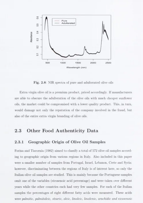
(w/w) sunflower oil and the final subsample is adulterated with 5% (w'/w) sunflower oil. Thus there are 138 spectroscopic scans in this study. The black lines (obscured) in Figure 2.8 are pure olive oil samples while the red lines are the olive oil samples th a t have been extended with sunflower oil. [image:30.513.11.506.60.590.2]P u r e A d u l t e r a t e d
C O o
o
500 1000 1500 2000 2500
W a v e l e n g t h ( n m )
F ig . 2.8: NIR spectra of pure and ad u lterated olive oils
E x tra virgin olive oil is a prem ium product, priced accordingly. If m anufacturers are able to obscure th e adu lteratio n of th e olive oils w ith much cheaper sunflower oils, the m arket could be com prom ised w ith a lower quality product. This, in turn, would dam age not only the rep u tatio n of th e com pany involved in th e fraud, but also of th e entire ex tra virgin branding of olive oils.
2.3
O th er F ood A u th e n tic ity D a ta
2.3.1
G eograp h ic O rigin o f O live Oil S am p les
Forina and Tiscornia (1982) aimed to classify a to tal of 572 olive oil samples accord ing to geographic origin from various regions in Italy. Also included in this paper were a smaller num ber of sam ples from P ortugal, Israel, Lebanon, C rete and Syria; however, discrim inating between the regions of Italy is of interest here, so only the Italian olive oil samples are studied. T his is m ainly because the Portuguese samples om it one of th e variables (eicosenoic acid percentage) and were taken over different years while th e other countries each had very few samples. For each of th e Italian samples th e percentages of eight different fatty acids were measured. These acids were palmitic, palmitoleic, stearic, oleic, linoleic, linolenic, arachidic and eicosenoic
[image:31.513.6.502.36.740.2]S ic ily S a rd in ia U m b ria A p u lia
L ig u ria C a la b ria
F ig . 2.9: M ap of Italy w ith th e regions of interest highlighted
T he regional breakdown of the d a ta is as follows: N orth A pulia (25 samples),
C alabria (56 sam ples), South A pulia (206 sam ples), Sicily (36 sam ples). Inland
Sardinia (65 sam ples). C oastal Sardinia (33 sam ples). E ast Liguria (50 samples).
West Liguria (51 samples) and 51 samples from Umbria.
G eographic origin is another factor th a t increases th e value of olive oil. This
extends further th a n ju st on a country level some regions w ithin Italy produce
olive oil th a t can be sold at a greater price th a n others. M isrepresenting th e region
of origin is thus not really a health and safety issue, rath e r a regulatory issue in
order to ])revent fraud and m aintain the prem ium value of p articu lar regions.
2.3.2
W in e
Forina et al. (1986) collected and analysed wine sam ples from the Piedm ont region
of Italy, which is to th e no rth of Liguria in Figure 2.9. T h e common, incom plete
d a ta set using only the inform ation abo ut alcohol, malic acid, ash content,
alcalin-ity, m agnesium content, total phenols, flavanoids, nonflavanoid phenols,
proantho-cyanins, intensity, hue, OD280/OD 315 o f phenols and proline is available in the
gclus (Hurley, 2004) package of R (R Developm ent Core Team , 2007).
For th e purposes of identifying wines solely into Barolo, Grignolino and Barbera
[image:32.513.16.507.49.669.2]1971, 1973-4; the 71 Grignoliiio wines are from th e years 1970-6 while the 48 B arbera
wines come from th e years 1974, 1976, 1978-9. Thus one cannot be certain th a t
discrim ination has not been m ade on the basis of year of production rath er th a n
solely by type, as intended. However, there is a significant difference in the price of
these wine varieties, hence th e m otivation for th e incorrect labelling.
W ith accurate inform ation on one variable unobtainable, th e rest of th e vari
ables associated w ith this wine d a ta are: sugar-free extract, fixed acidity, tartaric
acid, uronic acids, pH, potassium , calcium, phosphate, chloride, O D280/O D 315 of
flavanoidfi, (jlycerol, 2-3-lmtancdiol, total nitrocjcn and m,ethanol. Analysis is under
C hap ter 3
S ta tistica l M eth od ology
3.1
P a r tia l lea st squares reg ressio n
P a rtia l least squares discrim inant analysis is com monly used in food authentication
studies based on spectroscopic data. This m ethod uses p artial least squares regres
sion w ith a binary outcom e variable for two-group classification problem s and seeks
to optim ise b o th the variance explained and correlation w ith the response variable
(Ilastie et al., 2001, p66-p68). Downey et al. (2003) found it to outperform other
chem om etric m ethods commonly used in the stu d y of near infrared transfiectance
sp ectra such as Soft Independent Modelling of Class Analogies (SIM CA), which is
described in Section 3.2. It has th e advantage in th a t it can utilise highly-correlated
variables for classification purposes.
P a rtia l least squares regression (PLSR) was developed by Wold (1966a,6) and
is based on th e assum ption of a linear relationship between th e observed variables
(e.g. th e spectroscopy m easurem ents) and th e outcom e variable {e.g. pure or adul
terated ). It is sim ilar to principal com ponents regression (P C R ). Stone and Brooks
(1990) form ally explain th e connection between PLSR and PCR.
3.1.1
A lg o rith m for P L S R
As outlined by (H astie et al., 2001, p66-p68) each variable Xj is standardized to
have 0 m ean and variance of 1. T he response variable is y and p is th e num ber of
variables.
by Frank and Friedm an (1993). However an easier to follow version of the algorithm
was presented by H elland (1990) as follows:
1. Define startin g values for th e x residuals, e„,., and th e y residuals,
f„i'-(a) 6o X fix
(b)
f o = y - l-t-yFor 7)1 = 1 , 2 , . . .
2. The scores t are linear com binations of the x residuals from the last step
weighted by th e covariances w ith y residuals to m ake th e scores more closely
related to y:
(a) = C o v (e „ _ i, f m - i ) W j, Wa , . . . are orthogonal
( h ) t m =
3. L^etermine the x loadings, 1^, and y loading, <7,„, using least squares;
(a) I„j Cov(g^,_j , i^ )/V ar(/n ()
4. Find the new residuals
(a) Gtti
(b)
f m f m — 1 Qm — l i m —1It is further noted th a t the sequence of PLS coefficients for r/i = 1 , . . . , p represent
the conjugate gradient sequence for com puting least squares solutions.
3.1.2
N u m b er o f P a ra m eters
PLSR uses m relevant loadings/com ponents in the model. However, deciding on m
is not trivial as discussed by H elland (2001). Even when rn is known, th e num ber
of param eters in th e m odel is open for debate. Van Der Voet (1999) illustrated th e
problem in calculating the degrees of freedom of a model using PLSR. C alculating
penalty as p a rt of th e model selection criterion. For th e purposes of this thesis, the
num ber of param eters in th e population model was assum ed to be
So th a t if m = 0 no correlation between X and y exists and m = p is the full least
squares model; this agrees w ith Helland (2001).
3.2
Soft Independent M odelling o f Class A nalo
gies
Soft Independent M odelling of Class Analogies (SIMCA) was developed by Wold
(1976). T he underlying concept is to model each class separately using Principal
C om ponents (PC s). A different num ber of com ponents m ay be selected for each
class. In order to classify a new observation one of two approaches is then taken:
1. F ind th e M ahalanobis distance of th e new observation to each of th e existing
classes and place th e observation into th e “closest” class. Using this m ethod,
the probabilities of an observation belonging to each of th e groups can be
easily calculated.
2. C reate a set around each class developed in th e training set. If the new ob
servation falls w ithin these sets, it is then classified as belonging to this class.
T his m ethod can result in observations being classified into m ultiple classes,
a single class or no classes a t all and is quite a common approach used in the
chem om etrics literature.
M ore specifically: considering discrim inant analysis to use th e function
dg>(x) = mm [{x - Xg)'T,~'^{x - Xg) + log |Sg| - 2 log tt^]
w here Xg is th e m ean (vector) of th e variables associated w ith group g, Eg is the
covariance m atrix corresponding to group g and is the (prior) probability of an
observation belonging to group g. As Eg is a positive semi definite m atrix, it has
the sp ectral decom position:
V
where \ j g is the oigenvahie (in descending order) of Eg and ejg is the corre
sponding eigenvector.
If Sp is positive definite all of the A’s will be greater th a n 0 thu s can be
w ritten as
j=i
SIMCA instead uses
dg. {x) = rnm [(.x - X g)'E;^(Cg)(x - Xg)]
where
E
P f+ l 39
Z ^ j= C g + l '^39
For g = 1 , . . . , G th e num ber of principal com ponents, Cg, is estim ated using F
fold cross validation as outlined by (Wold, 1976,Section 2.2.1) T he cross validation
algorithm to im plem ent this m inim ization procedure is:
• For each group g — 1 , . . . , G:
• S te p 1: C reate the relevant subm atrix X g containing observations in the
training d a ta th a t belong to group g.
• S te p 2: Cross validation (w ithin each group g)\ For / = 1 , . . . F
• S te p 3: W ithhold observations in group g th a t belong to fold / to create X ~ ,
a m atrix w ith p variables and n “ observations. The w ithheld observations
are denoted as
• S te p 4: Find th e variable m eans of X ~ : X ~ .
• S te p 5: Find th e singular value decom position
where a = n “ — 1 if n “ < p or a = p if n ~ > p.
• S te p 6; (Jg is th e norm alised score m atrix, Vg th e loading m atrix and is
a diagonal m atrix containing th e singular values ordered so th a t Aig > \ 2g >
■ ■ ■ > ^ a g
-x„
• S te p 7: For r = 1 , . . . , a find Tg = — X ^ ) Vg (using th e first r cohunns
• S te p 8 : For each r find the sum of squares of th e residuals contained in each
of th e m atrices Eg's,
• S te p 9: If / < F , let / = / + 1 and retu rn to step 3.
num ber of com ponents to include for group g, call this Cg.
• S te p 11: If (/ < G, let g = g + 1 and retu rn to step 2.
• S te p 12: Now, for each group g th e num ber of com ponents Cg to include in
the model had been decided.
In m ethods where cross validation is designed to maximise classification perfor
m ance it has a tcndcncy to over-estim ate out of sam ple classification performance.
The selection criterion for the num ber of principal com ponents to use for each group
does not lend itself easily to use w ith Inform ation C riteria (such as BIC). Thus mod
els developed using th e SIMCA m ethod are not easily com pared to other commonly
used m ethods for near infrared spectroscopic data.
SIMCA effectively partition s the subspace. In th e i)rim ary sul)spac(; (first Cg
eigenvalues and eigenvectors) it assumes th a t th e eigenvalues of each group are
infinitely large so th a t l / \ j g = 0. In th e com plem ent of this space (of dimension
p — Cg), th e eigenvalues are estim ated by:
A lthough designed for large p small n problem s one of th e disadvantages of the
SIMCA m ethod is th a t it requires enough observations belonging to every group to
be included in th e train in g d a ta in order to use cross validation to select the num ber
of principal com ponents for each group. Therefore it is not suitable as a m ethod
where there are a large num ber of groups relative to th e num ber of observations in
the training data.
p x r
of Vg) and hence find th e value predicted object X g ^ = X ^ + Tg . Find
n j x r r x p
th e associated residuals Eg = X ^ — X g ^ .
• S te p 10: Choose the r th a t minimises Dr = determ ine the
When using a set to determ ine group m em bership ra th e r th a n th e relative prob
abilities of belonging to each group, m any observations m ay not be classified at all.
While placing an observation into m ultiple classes indicates uncertainty, b u t still
partially informs on th e decision process, failing to place an observation into any
group does not advance the knowledge abo ut th e sample. Assigning group mem
bership based on relative probabilities avoids this problem , b u t this also looses the
uniqueness of SIMCA as a m ethod. T h e tendency of SIMCA to classify observa
tions as outliers, thus not belonging to any group is exam ined for N IR spectra by
De Maesschalck et al. (1999).
Frank and Fiiedrnan (1989) proposes an am endm ent to this scheme Discrim
inant Analysis w ith Shrunken CO variances (DASCO), however this is not widely
used in the chem om etrics literatu re, thus not used as one of th e reference m ethods
w ithin this thesis.
3.3
L ik elih ood B a se d S ta tistic a l In feren ce
Likelihood based statistic al inference is based on th e prem ise th a t everything th a t
can be learned ab o u t th e param eters from th e d a ta is contained in the likelihood
function.
Suppose there is a sam ple X i , X2, . ■ ■, Xn where each observation is independently
generated from a d istribution. T he density of the observation can be w ritten
as J { x j \ 0 ) .
The (joint) density of th e whole sam ple is;
n
./(XnK^) =
. f { X i , X 2 - , . . . , X n \ 0 ) =J|/(.Tj|6')
j=lThe joint density is called th e likelihood function. T he jo in t density of th e data,
w ithout the condition of independence is a likelihood function, w ritten as:
L(0|x„) = /(x„|6>)
with unknown param eters 0. f is a function describing th e generating process of
M axim u m L ikelihood E stim a te (M LE)
Let L(0|x„) be the likeUhood function (defined for 9 € 0 ). A maximum hkehhood
estim ate is any vahie ^ € 0 for which L(^|x„) < L(^|x„) for all 9 E 0 .
However, it is often easier to maximise the log-likelihood function /(6^1x„) : =
logL(0|x„). As log is an increasing function so x > y logx > logy for x ,y > 0.
Thus an alternative expression for the MLE is Z(0|x„) > /(0|x„) V 9 G 0 . Suppose
th at the log-likelihood function /(0|x„) is a smooth function of 9. To maximise the
likelihood, differentiate the log-likelihood and solve for 9.
EM A lg o rith m
The Expectation Maximization (EM) algorithm (Dempster et al., 1977) was devel
oped as an iterative approach of calculating maximum likelihood estimates when
the observed d a ta could be considered to be incomplete. This incompleteness can
be introduced in order to simplify other calculations, or the unknown labels in a
clfissification problem can be considered as the missing data.
Given a joint distribution f { x , z\9) where x are observed variables, ^ are unob
served variables and 9 are parameters. The goal of the EM algorithm is to maximise
the likelihood function f {x\ 9) with respect to 9.
Let i = 0. Select a starting value for 9, 9^^\
Repeat
1. Estep: Evaluate f{z\x,9^*'^).
2. M step: Find = max^ Q(^|0W),
where Q{9\9^^^) = f { z \ x , 9^*'^) log f { x , z\9^^'>)dz.
3. t = i 1.
Until convergence.
The EM algorithm is relatively stable and simple to use as the Q function is
typically much simpler to maximise than f {x\ 6). However, it is not guaranteed to
3.4
M o d e l-b a se d D iscrim in a n t A n a ly sis
M odel-based discriminant analysis enables a better understanding of the generating
proccss that discrim inates between the different groups. It focuses on parameter
estim ation, finding a set of parameters that describe the source(s) o f separation
between groups.
In m odel-based discriminant analysis (also known as eigenvalue discrim inant
analysis) (Bensm ail and Celeux, 1996), the m odel is fitted to data w „ where n =
1 , 2 , . . . , and labels 1„ where Ing = 1 if observation n belongs to group g and 0
otherwise.
T he resulting likelihood function is
N G
>Cdi„c(Pl, P2, • • • , PG; 6'l, ^2, • • • , ^ g |w , 1) = ] ^ [Pgfi^n\ftg)]‘"^ ■ (3.1)
n=lg=l
The log of the likelihood function (3.1) is m axim ized yielding param eter estim ates
Pi) P2i ■ ■ ■iPg and 0i J) 2, . . . , Oq. For stabihty, equal probabilities, f>\ = ■■■= Pa =
1 /G , are som etim es assumed.
T he posterior probability o f group membership for an observation y whose label
is unknown can be estim ated as
P a f { y \ ^ 9 i
EJLi P<?/(y|^g)
P(Group g\ y ) « . (3.2)
Assum ing the density / to be a m ultivariate G aussian density, (f), w ith m ean fj.g
and covariance m atrix Eg
, , I ^ ^ e x p { - |( w „ . - /ig )^ E ;n w „ - fig)}
=
Tsmr)
■The m ultivariate G aussian densities im ply that the groups are centred at the means
fig w ith shape, orientation and volum e of the scatter of observations w ithin the
group depending on the covariance m atrices Eg.
T he parameters p and fi can then be estim ated by:
I
p { M ) ^ '"g if estim ated
V -v iV 1 - (fc+1) , 2 ^ n = l ^ n g ' ^ n
The Eg can be decomposed using an eigen decomposition into form,
= (3.3)
where Xg is a constant of proportionahty, Dg an orthogonal m atrix of eigenvectors
and Ag is a diagonal m atrix where the elements are proportional to the eigenvalues
as described by Fraley and Raftery (2002).
The estimates of Eg depend on the constraints placed on the eigenvalue decom
position; details of the calculations are given by Bensmail and Celeux (1996) and
Celeux and Govaert (1995).
The param eters Xg, Ag and Dg have interpretations in terms of volume, shape
and orientation of the scatter of the component. The param eter Xg controls the
volume while the matrices Ag and Dg control the shape of the scatter and the
orientation respectively. Constraining the parameters to be equal across groups
gives great modelling flexibility. Some of the options for constraining the covariance
param eters are given in Table 3.1 and are illustrated for the three group case by
Figure 3.1.
T a b le 3.1: Parametrizations of the covariance m atrix Eg
M o d e l ID D e c o m p o s itio n V o lu m e S h a p e O rie n ta tio n
E li Eg = A / Equal Identity Identity
V ll M II Variable Identity Identity
EEI Eg = A.4 Equal Equal Identity
VEI Eg = Ag.4 Variable Equal Identity
EVI Eg = A^lg Equal Variable Identity
VVI Variable Variable Identity
EEE Eg = X D A D ~ ^ Equal Equal Equal
EEV E g = X D g A D ^ Equal Equal Variable
VEV Variable Equal Variable
VVV ^9 ~ ^ g ^ g ^ g ^ J Variable Variable Variable
The letters in Model ID denote the volume, shape and orientation respectively.
For example, EEV represents equal vohune and shape with variable orientation. E li
[image:42.513.11.504.47.733.2]/ " " ^ i 1
V /
0
" °
A
v i * It ^ \\
'VM'O
0
r ' l
(p
- A
Fig. 3.1 : Possible combinations of volume, shape and orientation for 3 covariance
matrices
Model-bcised discriminant analysis is fitted to observations Wi, W2, . . . , Wtv by
maximizing the likehhood (3.1) using the EM algorithm (Dempster et al., 1977).
The resulting output from the EM algorithm includes estimates of the probability of
group membership for each observation; these can be used to cluster the observations
into their most probable groups.
The m clu st (Fraley and Raftery, 2007, 2002, 1999, 1998; Banfield and Raftery,
1993) package for R (R Development Core Team, 2007) can be used to perform
the model-based discriminant analysis. This allows for the possibility of the models
mentioned in Table 3.1. It is worth noting th at Linear Discriminant Analysis (LDA)
and Quadratic Discriminant Analysis (QDA) are special cases of model-based dis
criminant analysis and they correspond to the EEE and VVV models respectively.
3.4.1
U pdating
Model-based discriminant analysis as developed in Bensmail and Celeux (1996) only
uses the observations with known group membership in the model fitting procedure.
Once the model is fitted, the observations with unknown group labels can be clas
sified into their most probable groups.
An alternative approach is to model both the labelled d ata (w,l) and the unla
belled d ata y and to maximize the resulting log-likelihood for the combined model.
o b se rv a tio n s w ith in each group g are m odelled by a d e n sity f { - \ 9 g ) w here 9g are
unknow n p a ra m e te rs a n d t h a t th e p ro b ab ility of com ing from g roup g is pg.
G iven u n lab elled d a ta y w ith in d ep e n d e n t observ atio n s y i , . . . , Ym , a m ix tu re
m odel w ith C groups has a likelihood function
M G
H Y . ^ 3 f i y m \ 0 g ) - (3.4) m = l g = l
M axim ising e q u a tio n (3.4) using th e EM a lg o rith m (D e m p ste r et al., 1977) is th e
basis of m odel-b ased clu sterin g (Fraley a n d R aftery , 2002) a n d is easily im p lem en ted
in th e m c l u s t lib ra ry (Fraley a n d R aftery , 2007).
T h e likelihood function for th e com bined d a ta is a p ro d u c t of th e likelihood func
tio n s given in e q u a tio n s (3.1) a n d (3.4). T his classification a p p ro ach was developed
in D ean et al. (2006) a n d was d e m o n s tra te d to give im proved classification perfor
m an ce over th e classical m odel-based d isc rim in a n t an alysis in som e food a u th e n tic ity
a p p lic atio n s, using th e NIR m e a ts d a ta .
W ith th is m odelling ap p ro a c h th e likelihood fu n ctio n is of th e form
^ u p d a t e ( ? ^ )6 '|w ,l,y ) = £rti,,(/j,6i|w ,l)£.„i,(p,(9|y)
N G
nri[?'s./'(w„i6'p)]'"«
n = \ g = l
M G
n
^ P 9 . f g i y m \ 9 g_m = \ g = \
. (3.5)
T h e log of th e likelihood (3.5) is m axim ized using th e EM a lg o rith m to find esti
m a te s for p (if e stim a te d ) an d 6. O u tp u t from th e EM a lg o rith m includes e stim a te s
of th e p ro b a b ility of g roup m em bership for th e un lab elled o b serv atio n s y , as given
in e q u a tio n (3.2). In a p rac tic a l se ttin g , te s t set d a ta a re th e u n lab elled o b servations
w hile tra in in g d a ta are labelled observations.
T h e E M alg o rith m for m axim izing th e log of th e likelihood (3.5) proceeds ite r
a tiv e ly s u b s titu tin g th e u nknow n labels w ith th e ir e s tim a te d e x p e cte d values. A t
each ite ra tio n th e e stim a te d labels are u p d a te d a n d new p a ra m e te r e stim a te s are
p ro d u ced . By passing th e e stim a te d values of th e u nknow n labels in to th e EM algo
rith m it is possible to “u p d a te ” th e classification re su lts w ith som e of th e know ledge
g ained from fittin g th e m odel to all of th e d a ta . W ith sm all tra in in g se ts u p d a tin g
h as been show n to b e beneficial in o th e r stu d ies D ean et al. (2006), th u s th e p e r
form ance of u p d a tin g techniques were also included for ev a lu a tio n over o th e r N IR
U pdating techniques are especially useful when unlabelled observations can pro
vide useful inform ation abo ut separation betw'een groups. Figure 3.2 illustrates how
th e am ount of inform ation from an unlabelled observation can vary depending on
th e separation between th e group means. T he inform ation provided by unlabelled
observations decreases as the group means move closer together. T hus in Figure 3.2
points X, y and z are in the sam e positions, b u t th e am ount of inform ation they
provide ab ou t the groups varies according to th e separation between groups.
6
d
6
s6
•5 0 5
ei 6 o o 6 6 s o g 6 0 5 ■5 6 6 o 6 6 s6
-5 0 5
(a) (b) (c)
Fig. 3.2 : Means Separated by: 4 S tandard D eviations 3.2(a), 2 S tan dard Deviations
3.2(b) and 1 S tand ard D eviation 3.2(c)
3.4 .2
Im p lem en tin g th e E M A lg o rith m
T h e EM algorithm (D em pster et al., 1977) is ideally suited to th e problem of m axi
mizing the log-likelihood function w'hen some of the d a ta have unknowui group labels;
this arises in the m odel-based clustering likelihood (3.4) and the m odel-based dis
crim inant analysis w ith u pd atin g likelihood (3.5). In this section, th e steps involved
in the EM algorithm for m odel-based discrim inant analysis w ith u pd ating are illus
trated ; the m odel-based clustering steps are shown in Fraley and R aftery (2002).
Considering d a ta to be classified as consisting of M m ultivariate observations
consisting of two parts: known, and unknown z^ - In this context th e spectro
scopic d ata, which are observed and thus known, are tre a te d as th e y ^ - T he labels
(pure or ad ulterated ) are unknow n and th us are trea ted as the Zm- Additionally,
N labelled observations are available, which consist of two parts: known and