21 September 2011
first published online
, doi: 10.1098/rspa.2011.0137
468
2012
Proc. R. Soc. A
Antony A. Hill and M. S. Malashetty
coefficients
stability for systems with spatially dependent
An operative method to obtain sharp nonlinear
References
ated-urls
http://rspa.royalsocietypublishing.org/content/468/2138/323.full.html#rel Article cited in:
ml#ref-list-1
http://rspa.royalsocietypublishing.org/content/468/2138/323.full.ht
This article cites 19 articles, 3 of which can be accessed free
This article is free to access
Subject collections
(333 articles) applied mathematics
Articles on similar topics can be found in the following collections
Proc. R. Soc. A(2012)468, 323–336 doi:10.1098/rspa.2011.0137
Published online21 September 2011
An operative method to obtain sharp
nonlinear stability for systems with spatially
dependent coefficients
BY ANTONY A. HILL1,*AND M. S. MALASHETTY2
1School of Mathematical Sciences, University of Nottingham,
Nottingham NG7 2RD, UK
2Department of Mathematics, Gulbarga University, Jnana Ganga Campus,
Gulbarga 585106, India
This paper explores an operative technique for deriving nonlinear stability by studying double-diffusive porous convection with a concentration-based internal heat source. Previous stability analyses on this problem have yielded regions of potential subcritical instabilities where the linear instability and nonlinear stability thresholds do not coincide. It is shown in this paper that the operative technique yields sharp conditional nonlinear stability in regions where the instability is found to be monotonic. This is the first instance, in the present literature, where this technique has been shown to generate sharp thresholds for a system with spatially dependent coefficients, which strongly advocates its wider use.
Keywords: energy method; double-diffusive convection; porous media
1. Introduction
Two of the key techniques employed in a stability analysis are the nonlinear energy method and the more widely used method of linearized instability. A linear instability analysis, by definition, only provides boundaries for instability due to the presence of nonlinear terms (cf. Straughan 2004). The use of the energy method to construct stability thresholds is therefore crucial to assess whether the linear theory accurately encapsulates the physics of the onset and behaviour of an instability. Another key advantage of performing a nonlinear energy analysis is that it provides rigorous conditions for stability without exploiting linearization or weakly nonlinear approximations.
Nonlinear stability analyses have been performed successfully in a variety of applications, seeHill & Carr (2010)andSingh (2010). However, for a considerable range of problems, the standard energy approach does not generate sharp results (i.e. where the linear and nonlinear thresholds coincide), seeCarr (2003),
Sunil & Mahajan (2008) and Saravanan & Brindha (2010). This may, of course, be due to the significant possibility that the linear theory has not predicted
*Author for correspondence ([email protected]).
the onset of instability accurately; however, there are several new nonlinear energy techniques in development which show that sharp thresholds can still be achieved.
In the field of porous media convection, a differential constraint approach (cf. van Duijn et al. 2002) has been introduced, where the fluid-governing Darcy equation is retained as a constraint. This has been shown to reduce the number of required coupling parameters (cf. Hill 2009) and to provide sharp nonlinear thresholds in contrast to the standard approach, seeCapone et al.(2010).
In a separate recent development, an operative technique (for systems with constant coefficients) was introduced by Mulone (2004) that involves a change of variable in the energy method, based on the eigenvalues of the linearized system. In this paper, which was concerned with porous media convection, the coincidence of the critical linear and nonlinear stability parameters was proved. Further applications of this technique have seen sharp thresholds being produced for biological systems with diffusion (Mulone & Straughan 2009).
To assess the feasibility of an operative approach that could include systems with spatially dependent coefficients (which extends the use of the technique considerably), Hill (2008) further developed the method in the context of penetrative double-diffusive convection. This is an interesting test case, as the standard energy method approach yields a nonlinear threshold that is independent of the salt field. By adopting this new approach, a nonlinear threshold that was dependent on the salt field was shown, although coincidence between the linear and nonlinear thresholds was not achieved.
It is important to note that the operative technique yields regions of conditional stability, for which the initial data must be bounded by a threshold. Conditional stability does not necessarily preclude subcritical instabilities if this restriction on the initial data is not considered.
The purpose of this paper is twofold. Firstly, to improve on the design of the method from Hill (2008), now that its feasibility has been established, by basing the transformation solely on the linear eigenvalues, making the method much easier to solve numerically and, therefore, more widely useable. Secondly, to apply it to a physical system where all previous attempts to generate sharp nonlinear thresholds have not been successful in regions where the instability is monotonic. The technique, at present, has not been developed to be applicable in regions of oscillatory instability. The energy method itself (which underpins all of the nonlinear techniques) does not tend to generate sharp thresholds in such regions (cf.Straughan 2004). The operative technique will be used in conjunction with the differential constraint approach, which is a new development in the current literature.
Due to the competing temperature and salt gradients, double-diffusive convection poses a challenging nonlinear stability problem, and is therefore a good class of problems to test the method on. The introduction of a concentration-based internal heat source yields a system that forms an accurate model of cumulus convection as it occurs in the atmosphere (Krishnamurti 1997), and can also be interpreted as a simplified model of the salt gradient layer in a solar pond (Kudish & Wolf 1978). Although there has been considerable interest in this problem, see Krishnamurti (1997),Straughan (2002), Hill (2003,2005) and
differential constraint approach (Hill 2009). In this paper, we apply our operative technique to this problem (based on the results ofHill 2005), the purpose of which is to generate sharp nonlinear thresholds.
All numerical results were derived using the Chebyshev tau-QZ method (Dongarraet al.1996), which is a spectral method coupled with the QZ algorithm, and were checked by varying the number of polynomials to verify convergence.
2. Formation of the problem
Let us consider the same configuration as Hill (2005), where a fluid-saturated porous layer is contained between the horizontal parallel planes z=0 and L. Oxyz is the standard Cartesian frame of reference with unit vectors i,j and k, respectively. The model is of double-diffusive convection induced by the selective absorption of radiation, where the convection mechanism is essentially a penetrative one effectively modelled via an internal heat source.
The Darcy equation is assumed to govern the fluid motion in the layer, such that
m
Kv= −Vp−kgr, (2.1)
where v=(u,v,w) and p are velocity and pressure, g is the acceleration due to gravity, m is the dynamic viscosity of the fluid and K is the permeability.
Denoting T to be the temperature and C to be the concentration of the dissolved species, the density r(T,C) is given by
r(T,C)=r0(1−at(T −T0)+ac(C −C0)),
where r0, T0 and C0 are reference values of density, temperature and
concen-tration, respectively, and at and ac are the coefficients of thermal and solutal
expansion.
Equation (2.1), together with the incompressibility condition and the equations of energy and solute balance, yield the following system of governing equations:
m
Kv= −Vp−kgr0(1−at(T−T0)+ac(C −C0)), (2.2)
V·v=0, (2.3)
1
M
vT
vt +v·VT=ktDT+bC (2.4)
and 3vC
vt +v·VC=kcDC. (2.5)
The internal heat source is modelled linearly with respect to concentration, which is represented by the introduction of the bC term in equation (2.4), where b is some constant of proportionality. In these equations, 3 is the porosity, kt and kc
are the thermal and solutal diffusivities, andM=(r0hp)f/(r0h)m where (r0h)m=
(1−3)(r0h)s+3(r0hp)f, hp is the specific heat of the fluid and h is the specific
The boundary conditions for the problem are v=0, T=TL and C=CL at
z=0 andv=0,T=TU <TL,C=0 atz=L.
Assuming a steady-state solution (v,p,T,C) that corresponds to no fluid flow (i.e.v≡0), and introducing a perturbation to the steady state of the form
v=v+u, p=p+ ˆp, T=T +q and C=C +f, we may derive the governing non-dimensionalized perturbation equations,
u= −Vpˆ +kRT2q−kRS2Lef, (2.6)
V·u=0, (2.7)
vq
vt +u·Vq=wF(z)+Dq+tLef (2.8)
and fˆLevf
vt +Leu·Vf=w+Df. (2.9)
In these equations, Le=kt/kc is the Lewis number, fˆ=3M is the normalized porosity, t=bcLL2/(kt(TL−TU)) is a measure of the internal heat source generated by the radiation absorbing concentrate and R2T=
atgr0(TL−TU)KL/(mkt) andR2S=acgr0CLKL/(mkt) are the thermal and solute Rayleigh numbers, respectively. The term F(z)=1−t/3+t(z−z2/2) is the dimensionalized temperature gradient. Although a slightly different non-dimensionalization is used in this paper, a detailed derivation of equivalent governing equations and explicit parameter definitions may be found in Hill (2005).
The boundary conditions that follow from the perturbed quantities arew=0,
q=0 and f=0 at z=0, 1, where (u,q,f) have a periodic plan-form tiling the (x,y) plane, and U is the period cell for the perturbations.
3. Linear analysis
The linearized equations are derived from equations (2.6)–(2.9) by discarding the nonlinear terms. Introducing normal modes of the form
w=w(z) est+ia1x+ia2y, q=q(z) est+ia1x+ia2y and f=f(z) est+ia1x+ia2y,
wheres∈Cis the growth rate, and the wavenumbera2=a12+a22is a measure of the width of the convection cells that form at the onset of instability, and taking the doublecurl of equation (2.6) to remove the pressure term, system (2.6)–(2.9) yields
d2
dz2 −a 2
w+a2R2Tq−a2RS2f=0, (3.1)
d2 dz2 −a
2
q+wF(z)+tLef=sq (3.2)
and
d2
dz2 −a 2
with boundary conditions w=q=f=0 at z=0, 1. If Re(s)>0, then the perturbation will grow exponentially in time, clearly leading to linear instability. The sixth-order system (3.1)–(3.3) was solved using the Chebyshev-tau method (cf. Dongarra et al. 1996), which is a spectral technique coupled with the QZ algorithm. Numerical results for the linear theory are presented in §5.
4. An operative method approach to derive sharp nonlinear thresholds
The operative method approach that is used in this work is a development of the argument presented in Mulone (2004) (and later in Mulone & Straughan 2006) to address systems where the coefficients have spatial dependence. The presence of spatially dependent coefficients is highly common in double-diffusive porous convection problems, which makes this technique particularly applicable. A version of this technique was first applied to a simple penetrative double-diffusive convection problem in Hill (2008)to assess its feasibility.
(a)Transforming the nonlinear system
Our aim is to construct a transformation associated, in a canonical way, to the linear system via the first eigenvalue of the Laplacian operator that we can apply to our full nonlinear system (2.6)–(2.9).
However, in systems with spatially dependent coefficients (in our case, the
F(z) term in equation (3.2)), the eigenvalues of the Laplacian operator cannot be directly evaluated. To overcome this, we construct the transform based on the eigenvalues of a modified version of linearized equations. For equations (3.1)– (3.3), this is achieved by replacing F(z) with the average of its value over the range z∈ [0, 1] (namely 1).
Under this modified system, all the even derivatives of w,qand fnow vanish at the boundaries, so we may take solutions of the form
w=
∞
p=1
wp(t) sinppz, q=
∞
p=1
qp(t) sinppz and f=
∞
p=1
fp(t) sinppz.
It can easily be shown that the thermal Rayleigh number of this modified linearized system is minimized by the mode p=1. Since the sin functions are linearly independent, we may study only the most unstable mode p=1. Letting
s=aL2+p2 and a=aL2/(aL2+p2), equation (3.1) may be written
w=a(R2TLq−R 2
SLLef), (4.1)
where a2
L,R2TL and RSL2 are the wavenumber, and thermal and solute Rayleigh
numbers associated with the modified linear system, respectively. Using equation (4.1), the remaining linearized equations (3.2) and (3.3) may be written in the matrix form
X,t=MX,
where X=(q,f)T and
M= ⎛ ⎜ ⎝
−s+aR2TL −aLe R2SL+tLe
aR2TL
ˆ
fLe −
1 ˆ
f s
Le +R
2 SLa
The eigenvalues of matrixM are given by
eig(M)=1 2
a
R2TL−R
2 SL ˆ f −s 1 ˆ
fLe +1
±z2
, (4.2)
where
z1=a
RTL2 +
RSL2 ˆ f +s 1 ˆ
fLe −1
and z2=
z21+ 4aR 2 TL
ˆ
f (t−aR 2 SL).
Under the condition
z21+ 4aR 2 TL
ˆ
f (t−aR 2
SL)>0, (4.3)
the matrix Q of eigenvectors associated with eigenvalues equation (4.2) can be constructed, such that
Q= ⎛ ⎜ ⎝ ˆ fLe
2aRTL2 (z1+z2) ˆ
fLe
2aR2TL(z1−z2)
1 1
⎞ ⎟ ⎠
and
Q−1=
⎛ ⎜ ⎜ ⎜ ⎝
aRTL2 ˆ
fLez2
−z1+z2 2z2
− aR2TL
ˆ
fLez2
z1+z2 2z2 ⎞ ⎟ ⎟ ⎟ ⎠.
Introducing the new variables
g j
=Q−1
q f
,
we can now transform the full nonlinear system (2.6)–(2.9). Note that as all the values in the transformation are taken from the linear system (which are derived first), matricesQ and Q−1 contain only real numbers.
After making this substitution (and taking the third component of the double curl of equation (2.6) to remove the pressure term), we have the system
Dw=D∗(R2TQ11−Le R2S)g+D∗(R 2
TQ12−Le RS2)j, (4.4) vg
vt +(1+A1)u·Vg+A1u·Vj=F1w+(1+B1)Dg+B1Dj
+C1g+C1j (4.5)
and vj
vt +(1+A2)u·Vj+A2u·Vg=F2w+(1+B2)Dj+B2Dg
+C2g+C2j, (4.6) whereD∗=v2/vx2+v2/vy2 and
Aj=Qj2−1
1
ˆ
f−1
, Bj=Qj2−1
1
ˆ
fLe −1
Cj=tQj−11Le and Fj=F(z)Qj1−1+
Qj−21 ˆ
fLe,
with boundary conditions w=g=j=0 at z=0, 1.
(b)Deriving the sharp nonlinear stability bounds
To obtain sharp nonlinear stability bounds in the stability measure L2(U), (following an analogous argument to Lombardo et al. (2001)), we multiply equation (4.5) by g and Dg, respectively, and equation (4.6) by j and Dj, respectively, and integrate over U to obtain
1 2
d dtg
2+
A1u·Vj,g = F1w,g −(1+B1)Vg2−B1Vj,Vg
+C1g2+C1j,g,
−1 2
d dtVg
2+(1+A
1)u·Vg,Dg +A1u·Vj,Dg
= F1w,Dg +(1+B1)Dg2+B1Dj,Dg −C1Vg2−C1Vj,Vg,
1 2
d dtj
2+A
2u·Vg,j = F2w,j −(1+B2)Vj2−B2Vg,Vj
+C2g,j +C2j2
and −1
2 d dtVj
2+
(1+A2)u·Vj,Dj +A2u·Vg,Dj = F2w,Dj
+(1+B2)Dj2+B2Dg,Dj −C2Vg,Vj −C2Vj2,
where · and ·,· denote the norm and inner product on L2(U). Adopting
the differential constraint approach of van Duijn et al. (2002) and Hill (2009), equation (4.4) is retained as a constraint. This is the first instance, in the current literature, in which the differential constraint approach has been used in conjunction with an operative method.
Letting
E(t)=1 2(g
2+
lj2)+b 2(Vg
2+
Vj2),
where l>0 is a coupling parameter, andb is a positive constant, we can write
dE
dt =I0−D0+N0+bI1−bD1+bN1, (4.7)
where
I0= F1w,g +lF2w,j +C1g2+lC2j2
+(C1+lC2)j,g −(B1+lB2)Vj,Vg,
N0= −A1u·Vj,g −lA2u·Vg,j,
I1= −F1w,Dg − F2w,Dj +C1Vg2+C2Vj2
+
1− 1
ˆ
fLe
Dj,Dg,
D1=(1+B1)Dg2+(1+B2)Dj2
and N1= −(1+A1)u·Vg,Dg −A1u·Vj,Dg
−(1+A2)u·Vj,Dj −A2u·Vg,Dj.
To ensure thatD0,D1>0 (i.e. 1+B1>0 and 1+B2>0), we have the condition
4fˆLe
(fˆLe+1)2z 2 1+
4aR2TL ˆ
f (t−aR 2
SL)>0. (4.8)
Note that if equation (4.8) holds, then condition (4.3) follows. By defining
D2=
RE −1 2RE
D0+
b
2D1 with 1
RE
=max
H I0
D0 ,
whereH is the space of admissible functions, it follows that bI1≤D2 and N0+
bN1≤p1D2E1/2 for a positive constantp1 (see appendix A), where RE>1. From equation (4.7), we see that
dE
dt ≤ −D2(1−p1E
1/2).
If RE>1, then by the Poincaré inequality (e.g. p2g2≤ Vg2), D2≥p2E for some positive constantp2. Hence, it follows that
dE
dt ≤ −p2E(1−p1E
1/2
). (4.9)
We will show that equation (4.9) ensures conditional nonlinear stability as long as
RE>1 (4.10a)
and
E1/2(0)< 1
p1
. (4.10b)
For equation (4.10b) to hold, there are two possibilities as follows:
(i) E1/2(t)<1/p1, t≥0,
or
(ii) there exists z>0 such that E1/2(z)=1/p1, with E1/2(t)<1/p1, for
Suppose (ii) holds. From equation (4.9), it follows that dE/dt≤0 for t∈ [0,z), hence,E1/2(t)≤E1/2(0)<1/p
1for anyt∈ [0,z). AsE(t) is a continuous function of t on[0,z], then it is impossible thatE1/2(z)=1/p1. This contradiction implies (i) and consequently dE/dt≤0 fort≥0 such thatE1/2(t)≤E1/2(0). Thus,
dE
dt ≤ −p2(1−p1E
1/2 (0))E.
Integrating, we have
E(t)≤E(0) e−p2(1−p1E1/2(0))t→0 ast→ ∞,
which shows the decay ofg andj. Using equation (2.6),
u ≤ |RT2Q11−R2SLe|g + |R 2
TQ12−R2SLe|j. (4.11)
The decay of u clearly follows.
It is important to note that we have derived conditional stability (under the restriction (4.10b)), such that the initial dataE1/2(0) must be bounded by 1/p1. From the definition of p1 (see appendix A) as RE→1, the bound on the initial data tends to 0. However, forfˆ=1, we may takeb=0, which yields unconditional nonlinear stability, such that there is no bound on the initial data.
Following the differential constraint approach of van Duijn et al. (2002) and
Hill (2009) (where we retained equation (4.4) as a constraint), we introduce an Euler–Lagrange multiplier m such that
m(x)(Dw+D∗(Le R2S−R 2
TQ11)g+D∗(Le R2S−R 2
TQ21)j)=0.
The Euler–Lagrange equations for the maximization problem 1/RE =
maxH(I0/D0) are now given by
RE(Dw+D∗(Le R2S−R 2
TQ11)g+D∗(Le R2S−R 2
TQ21)j)=0,
RE(Dm+F1g+F2lj)=0,
RE(F1w+(C1+lC2)j+2C11g+(B1+lB2)Dj
+(Le R2S−R2TQ11)D∗m)+2(1+B1)Dg=0 (4.12)
and RE(lF2w+(C1+lC2)g+2C2lj+(B1+lB2)Dg
+(Le R2S−R 2
TQ12)D∗m)+2(1+B2)Dj=0,
with boundary conditions w=m=g=j=0 at z=0, 1.
After adopting normal modes, the eighth-order eigenvalue problem (4.12) for
RE was solved using the Chebyshev-tau method (cf.Dongarraet al.1996). Under
the analysis of this section, the ranges of the remaining parameters (restricted by equation (4.8)) with eigenvaluesRE>1 correspond to regions of stability. An
5. Results and conclusions
For fixed values of Le, t, fˆ and R2
S, the region (in terms of R 2
T) that yielded conditional stability under the operative method was numerically derived by adopting the following approach:
(1) solve the linear instability problem to yield the critical values ofR2 TL and
a2
L (noting that R 2 SL=R
2 S);
(2) if condition (4.8) is satisfied, then the nonlinear operative approach may be applied;
(3) use the derived R2TL and aL2 values to define the constants Aj,Bj, Cj and the functions Fj (j=1, 2) in equation (4.12);
(4) fix the value ofR2T;
(5) minimizeRE over the wavenumbera2and maximizeRE over the coupling parameterl by repeatedly solving eigenvalue problem (4.12) forRE; (6) ifRE>1, then we have stability; and
(7) repeating steps 5 and 6 for a variety of RT2 values yields the region of stability.
Eigenvalue problem (4.12) was solved using the Chebyshev tau-QZ method (Dongarra et al. 1996), which is a spectral method coupled with the QZ algorithm. The results were checked by varying the number of polynomials to verify convergence. To compare our operative technique with the existing energy methods, standard nonlinear stability results are also derived (see Hill 2005 for more details).
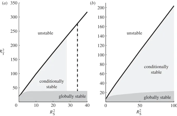
Figure 1 presents stable and unstable regions, which have been generated numerically, in a graphical form. As the linear instability thresholds (which give the unstable regions) have been presented before for a range of parameter values in Hill (2005), figure 1 simply gives a representative example of how the operative method performs. The conditionally stable and globally stable regions correspond to the results generated by the operative and standard nonlinear stability approaches, respectively.
It is immediately obvious fromfigure 1 that the operative technique produces sharp thresholds. In figure 1a,b, as RS2 is increased, the region between the linear and standard nonlinear thresholds becomes very substantial. This region is entirely removed by the operative approach, clearly demonstrating the highly substantial improvement this new technique brings over the existing methods.
However, in contrast to the operative method, the standard approach yields unconditional stability (such that there is no bound on the initial data). The conditional stability generated by the operative approach does not necessarily preclude sub-critical instabilities if the restriction on the initial data is not considered.
0 10 20 30 40 50
100 150 200 250 300
unstable
globally stable conditionally
stable 350
(a) (b)
0 50 100
20 40 60 80 100 120 140 160 180 200
unstable
conditionally stable
globally stable
R2
T
[image:12.493.79.423.57.283.2]R2S R2S
Figure 1. Visual representation of unstable, conditionally stable (nonlinear operative method) and globally stable (standard nonlinear method) regions, with critical thermal Rayleigh number R2T
plotted against R2S. The solid line represents the onset of linear instability, such that the region above it is unstable. The dashed line represents the point at which the transformation is no longer valid for increasing RS2. The graphs correspond to (a) t=1,fˆ=0.1,Le=20 and (b) t=5,fˆ=
0.1,Le=20.
It has been demonstrated that for a system with spatially dependent coefficients, the operative technique presented in this paper can generate sharp thresholds, which is not achieved by the standard approach. This strongly advocates its wider use, with the potential to sharpen nonlinear stability thresholds in a substantial number of problems. The stability results generated by this approach are conditional, though, such that the initial data must be bounded by a defined threshold.
The authors would like to thank three anonymous referees whose comments have led to improvements in the paper.
Appendix A
Recall that for RE>1 andb>0,
D0=(1+B1)Vg2+l(1+B2)Vj2, D2=
RE−1 2RE
D0+
b
2D1,
D1=(1+B1)Dg2+(1+B2)Dj2
and I1= −F1(z)w,Dg − F2(z)w,Dj +C1Vg2+C2Vj2
+
1− 1
ˆ
fLe
Dj,Dg,
Lettingg1=maxz∈[0,1]F12(z) andg2=maxz∈[0,1]F22(z), using Young’s inequality (for constantsc1,c2>0) and noting thatC2<0, it follows that
bI1≤
b 2 1 c1 + 1 c2
w2+bC1Vg2
+b
2
c1g1+1− 1
ˆ
fLe
Dg2+
c2g2+1− 1
ˆ
fLe
Dj2
.
Choosingc1and c2 such that
c1g1+1− 1
ˆ
fLe =1+B1 and c2g2+1−
1
ˆ
fLe=1+B2,
which holds for 1<fLe<3, we have
bI1≤
b
2
g1fˆLe
B1fˆLe+1
+ g2fˆLe
B2fˆLe+1
w2+bC1Vg2+
b
2D1.
Using equation (4.11) yields
bI1≤
b
2c5(c3+c4)(c3g 2+c
4j2)+bC1Vg2+
b
2D1,
where
c3= |RT2Q11−R2SLe|, c4= |RT2Q12−R2SLe|
and c5=
g1fˆLe
B1fˆLe+1
+ g2fˆLe
B2fˆLe+1 .
Using the Poincaré inequality and letting
b=
RE−1
RE
min
(1+B1)p2
c3c5(c3+c4)+2C1p2
, l(1+B2)p 2
c4c5(c3+c4)
,
we have
bI1≤
RE−1 2RE
D0+
b
2D1=D2,
as required.
ConcerningN0, using the inequality supU|f| ≤c6Df, where
c6=
√
3
(p5h3√2(√2−1))1/2+
25/25(1+p2)1/2h3/5
and f =0 on z=0, 1, (cf. Straughan 2004), the Cauchy–Schwarz inequality and equation (4.11), we have
N0= −A1u·Vj,g −lA2u·Vg,j
≤ |A1|c6DguVj +l|A2|c6DjuVg
≤c6(c3g +c4j)(|A1|DgVj +l|A2|DjVg)
≤c6
c3
√
2E1/2+c4
2
lE
1/2 2|
A1|D2
RE
lb(1+B1)(1+B2)(RE −1)
1/2
+2l|A2|D2
RE
b(1+B1)(1+B2)(RE −1)
1/2
≤r1E1/2D2,
where
r1=23/2c6
RE
b(1+B1)(1+B2)(RE−1)
1/2
c3+
c4
√
l
|A1|
√
l +l|A2|
.
It is important to note that r1→ ∞ asRE→1.
Again, using the inequality supU|u| ≤c6Du, the Cauchy–Schwarz inequality
and equation (4.11), we obtain
bN1= −b(1+A1)<u·Vg,Dg>−bA1<u·Vj,Dg>
−b(1+A2)<u·Vj,Dj>−bA2<u·Vg,Dj>
≤bc6(c3Dg +c4Dj)(|1+A1|VgDg + |A1|VjDg
+ |1+A2|VjDj + |A2|VgDj)
≤r2E1/2D2,
where
r2=
2√2c6
√
b
c3
√ 1+B1
+ c4
√ 1+B2
|1+A1| + |A1|
√ 1+B1
+|1+A2| + |A2|
√ 1+B2
.
Hence,
N0+bN1≤p1D2E1/2,
where p1=max(r1,r2), as required, withp1→ ∞asRE→1.
References
Capone, F., Gentile, M. & Hill, A. A. 2010 Penetrative convection via internal heating in anisotropic porous media.Mech. Res. Comm.37, 441–444. (doi:10.1016/j.mechrescom.2010.06.005) Carr, M. 2003 A model for convection in the evolution of under-ice melt ponds. Contin. Mech.
Thermodyn.15, 45–54. (doi:10.1007/s00161-002-0103-3)
Chang, M. H. 2004 Stability of convection induced by selective absorption of radiation in a fluid overlying a porous layer.Phys. Fluids16, 3690–3698. (doi:10.1063/1.1789551)
Hill, A. A. 2003 Convection due to the selective absorption of radiation in a porous medium.
Contin. Mech. Thermodyn.15, 275–285. (doi:10.1007/s00161-003-0115-7)
Hill, A. A. 2005 Double–diffusive convection in a porous medium with a concentration based internal heat source.Proc. R. Soc. A461, 561–574. (doi:10.1098/rspa.2004.1328)
Hill, A. A. 2008 Global stability for penetrative double-diffusive convection in a porous medium.
Acta Mech.200, 1–10. (doi:10.1007/s00707-007-0575-0)
Hill, A. A. 2009 A differential constraint approach to obtain global stability for radiation induced double-diffusive convection in a porous medium.Math. Meth. Appl. Sci. 32, 914–921. (doi:10.1002/mma.1073)
Hill, A. A. & Carr, M. 2010 Nonlinear stability of the one-domain approach to modelling convection in superposed fluid and porous layers. Proc. R. Soc. A 466, 2695–2705. (doi:10.1098/rspa.2010.0014)
Krishnamurti, R. 1997 Convection induced by selective absorption of radiation: a laboratory model of conditional instability. Dynam. Atmos. Oceans 27, 367–382. (doi:10.1016/ S0377-0265(97)00020-1)
Kudish, A. I. & Wolf, D. 1978 A compact shallow solar pond hot water heater.Sol. Energy 21, 317–322. (doi:10.1016/0038-092X(78)90008-7)
Lombardo, S., Mulone, G. & Straughan, B. 2001 Non-linear stability in the Bénard problem for a double-diffusive mixture in a porous medium. Math. Meth. Appl. Sci. 24, 1229–1246. (doi:10.1002/mma.263)
Mulone, G. 2004 Stabilizing effects in dynamical systems: linear and nonlinear stability conditions.
Far East J. Appl. Math.15, 117–134.
Mulone, G. & Straughan, B. 2006 An operative method to obtain necessary and sufficient stability conditions for double diffusive convection in porous media. ZAMM 86, 507–520. (doi:10.1002/zamm.200510272)
Mulone, G. & Straughan, B. 2009 Nonlinear stability for diffusion models in biology.SIAM J. Appl. Math.69, 1739–1758. (doi:10.1137/070697884)
Saravanan, S. & Brindha, D. 2010 Global stability of centrifugal filtration convection.J. Math. Anal. Appl.367, 116–128. (doi:10.1016/j.jmaa.2009.12.026)
Singh, J. 2010 Energy relaxation for transient convection in ferrofluids.Phys. Rev. E 82, 026311. (doi:10.1103/PhysRevE.82.026311)
Straughan, B. 2002 Global stability for convection induced by absorption of radiation.Dynam. Atmos. Oceans35, 351–361. (doi:10.1016/S0377-0265(02)00051-9)
Straughan, B. 2004The energy method, stability and nonlinear convection. New York, NY: Springer. Sunil & Mahajan, A. 2008 A nonlinear stability analysis for magnetized ferrofluid heated from
below.Proc. R. Soc. A464, 83–98. (doi:10.1098/rspa.2007.1906)