Modern Robust Statistical Methods: Basics
with Illustrations Using Psychobiological Data
Rand R. Wilcox
1,∗,
Douglas A. Granger
2,
Florence Clark
31Dept. of Psychology, University of Southern California, Los Angeles, CA 90089-1061, United States
2Center for Interdisciplinary Salivary Bioscience Research, Johns Hopkins University,
School of Nursing, Bloomberg School of Public Health, and School of Medicine
3Division of Occupational Science & Occupational Therapy, University of Southern California
∗Corresponding Author: [email protected]
Copyright c⃝2013 Horizon Research Publishing All rights reserved.
Abstract
Psychological studies in general, and psychobiological studies in particular, routinely use a collection of classic statistical techniques aimed at comparing groups or studying associations. A funda-mental issue is whether violating the basic assumptions underlying these methods, namely normality and homoscedasticity, can result in relatively poor power or miss important features of the data that have practical significance. In the statistics literature, hundreds of papers make it clear that under general conditions the answer is yes and that routinely used strategies for dealing with violations of assumptions can be unsatis-factory. Moreover, a vast array of new and improved techniques is now available for dealing with violations of assumptions, including more flexible methods for dealing with curvature. The paper reviews the major insights regarding standard methods, explains why some seemingly reasonable methods for dealing with violations of assumptions are technically unsound, and then outlines methods that are technically correct. It then illustrates the practical importance of modern methods using data from the Well Elderly II study.Keywords
Psychobiological studies, robust statis-tical methods, outliers, curvature, heteroscedasticity, smoothers, biomarkers, depressive symptoms, meaning-ful activity1
Introduction
Classic statistical techniques, routinely used in psy-chological studies, are based in part on two basic as-sumptions: normality and homoscedasticity (equal vari-ances). A well-known view is that these techniques are robust when either of these assumptions is violated. But it is well known in the statistics literature that, un-der general conditions, commonly used methods can be highly unsatisfactory (e.g., [18, 21, 22, 36, 38, 42, 43] It is evident, however, that psychobiological studies do not
take the advances and insights into account.
Briefly, standard methods are robust in terms of Type I errors when comparing groups that have identical dis-tributions, or when dealing with regression and the vari-ables under study are independent. So a positive feature of classic methods based on means is that if they yield a significant result, it is reasonable to conclude that dis-tributions differ in some manner. And if when using Pearson’s correlation, if Student’s t rejects, it is reason-able to conclude that there is some type of association. Of course, if distributions differ or there is an associa-tion, standard methods might continue to perform well in terms of power, accurate confidence intervals, as well as providing a reasonable characterization of how groups differ or the association among variables. But to assume that these methods perform in a relatively effective man-ner is not supported by hundreds of published papers. Transforming data is a well-known strategy for dealing with violations of assumptions, but by modern standards this approach is relatively ineffective for reasons that are reviewed and illustrated.
2
Summary of Three Major
In-sights
As previously indicated, there have been three major insights regarding classic methods based on means and the least squares regression estimator. Briefly, they deal with 1) the impact of heavy-tailed distributions and out-liers, 2) skewed distributions and the central limit the-orem, and 3) heteroscedasticity. The immediate goal is to describe and illustrate each of these issues.
2.0.1 Heavy-tailed Distributions and Outliers
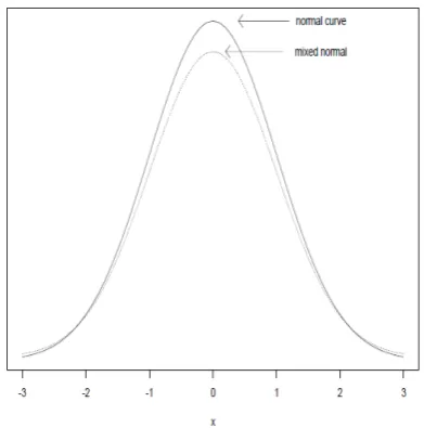
[image:2.595.315.517.89.283.2]A small departure from a normal distribution can have a large impact on the population variance, which in turn could mean relatively poor power when compar-ing means. A classic illustration stems from the mixed (or contaminated) normal distribution as discussed by Tukey (1960). The particular mixed normal distribu-tion he considered is a situadistribu-tion where with probability 0.9 an observation is sampled from a standard normal, otherwise an observation is sampled from a normal dis-tribution with mean 0 and standard deviation 10. Fig-ure 1 shows the standard normal distribution, which of course has variance one, and the mixed normal. Despite the obvious similarity between the two distributions, the mixed normal has variance 10.9. The mixed normal is an example of a heavy-tailed distribution meaning that the tails are thicker than a normal distribution.
Figure 1. Shown are the standard normal and mixed normal distributions. Despite the obvious similarity between the two dis-tributions, the variance of the mixed normal is 10.9
Figure 2 illustrates the impact of a heavy-tailed tribution on power. In the left panel are two normal dis-tributions, each having variance one with means equal to 0 and 1. The power of Student’s t, when testing at the .05 level and with sample sizes of 25 per group, is .96. But in the right panel, which shows two mixed nor-mals, again having mean 0 and 1, power is only .28. Put another way, random samples from heavy-tailed distri-butions are characterized by outliers and even a single outlier has the potential of inflating the sample variance, which in turn can result in poor power. The presence of outliers does not necessarily spell disaster, but
sim-ply ignoring the potential impact of outliers cannot be recommended.
Figure 2. In the left panel, power is .96 when using Student’s t withn= 25 and when testingat the .05 level. But in the right panel, power is only .28
2.0.2 Skewed Distributions and the Central Limit Theorem
Next consider the central limit theorem. A common misconception is that with a sample size of 25 or more, normality can be assumed. So in particular,
T = ¯
X−µ s/√n
is assumed to have a Student’s t distribution withn−1 degrees of freedom, wherenis the sample size, ¯X is the usual sample mean andµis the population mean. This view stems from studies where sampling is from light-tailed distributions, roughly meaning that outliers are relatively rare. However, these early results missed two fundamental points. The first has to do with situations where a skewed distribution tends to have outliers. Now, more than 100 observations might be needed so that the sample mean has, approximately, a normal distribution. Second, and perhaps more importantly, is the implicit assumption that if the sample mean has a normal distri-bution, Student’s t will be reasonably accurate in terms of Type I error probabilities and confidence intervals. Even with a skewed, light-tailed distribution, where the sample mean has approximately a normal distribution, a sample size of over 200 might be needed to get accurate results when using Student’s t (e.g., [41, 42, 43]. For a skewed, heavy-tailed distribution (outliers are com-mon), a sample size of 300 or more might be needed (e.g., [42, 43].
[image:2.595.65.261.416.614.2]older people. One of the variables was salivary cortisol upon awakening, 30-60 minutes later, 5 hours later, and 5 hours later. Cortisol has been found to be associ-ated with various measures of psychological stress and is generally considered to be a valuable marker of the hypothalamus-pituitary-adrenal (HPA) axis (e.g., [15]). Compliance with the sampling schedule was monitored by recording the times when the sample was taken. Sam-ples were assayed for cortisol using a highly sensitive en-zyme immunoassay without modifications to the manu-facturers recommended protocol (Salimetrics, State Col-lege, LLC). The test uses 25ul test volume, ranges in sen-sitivity from .007 to 3.0 ug/dl, and has average intra- and inter-assay coefficients of variation of 4.13% and 8.89%, respectively.
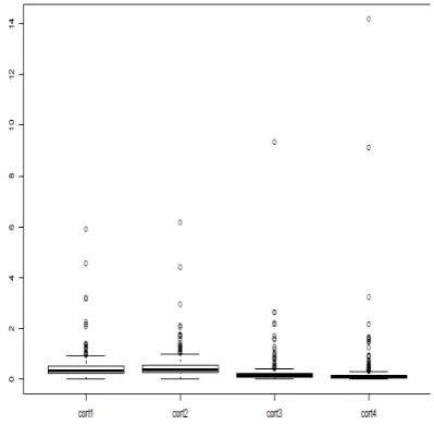
[image:3.595.328.532.153.345.2]Figure 3 shows a boxplot of the cortisol data. As is ev-ident, at all four times, the data are skewed with outliers. Boxplots for DHEA (dehydroepiandrosterone), which is also considered to be a valuable marker of the HPA axis, and salivary alpha amylase, not shown here, are similar to those in Figure 3. (Salivary secretion of alpha amy-lase has been proposed as an indicator of plasma cat-echolamine modifications under a variety of conditions. Catecholamines play an important role in the body’s physiological response to stress.)
Figure 3. Boxplots of salivary cortisol measured at four different times during the day
The skewed distribution in Figure 4 is a bootstrap-t approximabootstrap-tion of bootstrap-the disbootstrap-tribubootstrap-tion of T based on the cortisol data upon awakening. Based on a sample of
nobservations, the bootstrap-t method randomly sam-ples with replacementnobservations from the observed data, computesT and then repeats thisB times. Here,
B = 2000 was used. (In effect, perform a simulation study on the observed data.) Also shown is the distri-bution of T under normality. As can be seen the left tails differ substantially despite having a sample size of
n = 254. Under normality, when testing a two-sided hypothesis at the .05 level, the lower .025 critical value would be−1.97. But the approximation indicates that it should be−3.03. Put another way, if we assume normal-ity and reject whenT is less than−1.97, the probability of a Type I error, when the null hypothesis is true, is .025. But the approximation indicates that the actual
Type I error probability is .071, nearly three times larger than intended. In the right tail we see the opposite prob-lem. The probability of rejecting is estimated to be .008, substantially less than the intended level of .025, which has implications about low power when the null hypoth-esis is false and the actual value ofµis greater than the hypothesized value.
Figure 4. The approximate distribution of Student’s t based on awakening cortisol,n= 254
A valid criticism of this illustration is that the bootstrap-t approximation of the distribution ofTmight be inaccurate. Results summarized in [43] indicate that indeed there are practical concerns: problems with Stu-dent’s t are probably worse than indicated. In particu-lar, in all likelihood, the left tail does not extend out far enough and the actual Type I error is most likely higher than indicated. The bootstrap-t method can improve control over the Type I error probability, but in general practical problems remain.
In the Well Elderly II study, measures were taken again six months after intervention. Boxplots of cor-tisol, DHEA and alpha amylase are similar to those in Figure 3. For cortisol measured upon awakening, the Type I error probability was estimated to be .086 for the lower tail when testing at the .025 level, using Stu-dent’s t, and for the upper tail it was estimated to be .004. So for a two-sided hypothesis, the estimate is that when testing at the .05 level, the actual level is .090 and it is probably higher based on known results regarding the bootstrap-t approximation that was used.
[image:3.595.76.276.370.565.2]skew-ness, illustrate that now control over the Type I error probability can be unsatisfactory. In practical terms, if the goal is to test the hypothesis of identical distribu-tions, Student’s t is satisfactory in terms of controlling the probability of a Type I error. It might provide accu-rate information about the population mean, but under general conditions this is not the case.
2.0.3 Heteroscedasticity
When using a hypothesis testing method that assumes homoscedasticity, heteroscedasticity further exacerbates the problems already described and illustrated. One ba-sic reason is that under general conditions, if there is heteroscedasticity, homoscedastic methods are using the wrong standard error. Cressie and Whitford (1986) de-scribe general conditions where, when comparing two independent groups, Student’s t is not even asymptoti-cally correct. That is, when testing at the .05 level, for example, a basic requirement of any method is that the actual Type I error probability should converge to .05 as the sample size gets large. But under general conditions, Student’s t does not enjoy this property. Moreover, the more complicated the design, the more serious are prob-lems associated with heteroscedasticity when using a homoscedastic method (e.g., Wilcox, 2012a). For ex-ample, under normality, when comparing two indepen-dent groups, Stuindepen-dent’s t controls the probability of a Type I error reasonably well when equal sample sizes are used. But for the ANOVA F test, when comparing four groups, this is no longer the case. Again, if the goal is to test the hypothesis that groups have identical dis-tributions, Type I errors are controlled reasonably well via the ANOVA F test. But if the goal is to control Type I errors when testing the hypothesis of equal means, the ANOVA F test can be highly unsatisfactory.
3
Some Unsatisfactory Strategies
3.0.4 Detecting Outliers
When checking for outliers, methods based on the mean and standard deviation are known to be highly unsatisfactory because this approach results in masking, roughly meaning that the very presence of outliers can cause them to be missed (e.g., [36, 42]). Briefly, outliers inflate the sample variance so that even extreme out-liers can be missed. For univariate data there are two basic outlier detection techniques that avoid masking. The first is a boxplot and the other is the MAD-median rule. To describe the MAD-median rule, letX1, . . . , Xn
be n observations and let M be the usual sample me-dian. The median absolute deviation (MAD) is equal to the median of|X1−M|, . . . ,|Xn−M|. It represents
a measure of variation that is insensitive to outliers, a key feature needed to avoid masking. The MAD-median rule declares the valueX an outlier if
|X−M|
MAD/.6745 >2.24.
(Under normality, MAD/.6745 estimates the usual pop-ulation standard deviation.) Compared to the boxplot, the MAD-median rule is better at avoiding masking.
Nevertheless, there are practical reasons for still using a boxplot, but the details go beyond the scope of this review. For multivariate data, Mahalanobis distance is unsatisfactory as well: it suffers from masking. For a recent summary of more satisfactory methods for de-tecting multivariate outliers, see Wilcox (2012b).
3.0.5 Dealing with Heterosecedasticity
A seemingly natural strategy for dealing with het-erosecedasticity is to test the hypothesis that there is homoscedasticity and use a homoscedastic method if a non-significant result is obtained. However, five pub-lished papers (summarized in Wilcox, 2012a) have stud-ied this strategy and all five came to the same conclu-sion: this approach is unsatisfactory. The simple ex-planation is that the power of the methods used to test the homoscedasticity assumption is not high enough to detect situations where the assumption should be aban-doned. Currently, a better strategy is to always use a method that allows heterosecedasticity. Little is lost if in fact there is homoscedasticity, but much can be gained in terms of accurate probability coverage and power. This remains the case when dealing with regression [26].
3.0.6 Transforming Data
There are two fundamental limitations regarding sim-ple transformations (e.g., [8, 33]. First, transforming data does not deal effectively with outliers. In some sit-uations the number of outliers is decreased, but in other situations the number stays about the same and can even increase. The fact that even a single outlier might re-sult in poor power renders simple transformations to be an effective method. Second, typically, but not always, distributions remain substantially skewed.
Consider again the cortisol data in Figure 3. Taking logs, the number of outliers drops from 19 to 13 and a boxplot again indicates a skewed distribution. So a pos-itive feature of taking logs is a reduction in the number of outliers. But a serious concern is that outliers remain that can negatively impact power. And it is unclear that problems associated with skewed distributions have been adequately addressed.
3.0.7 Discarding Outliers and Applying Meth-ods for Means Using the Remaining Data
but they are not remotely obvious based on standard training.
4
Technically Sound Methods for
Dealing with Skewed
Distribu-tions and Outliers
There are several ways of dealing with skewed distri-butions and outliers in a technically sound manner with each being sensitive to different features of the data and providing different perspectives on how groups compare and how variables are related.
4.0.8 The Median and Trimmed Means
One possibility is to compare groups using the usual sample median. It is highly insensitive to outliers be-cause after putting observations in ascending order, all but one or two values are trimmed. Also, if the goal is to characterize the typical response, the median is ar-guably a better choice than the mean when dealing with a skewed distribution. However, a concern is that be-cause the usual sample median trims nearly all of the observations, power might be relatively low. This is the case under normality. But even two centuries ago, Laplace was aware of conditions where the median has a smaller standard error than the mean (Hand, 1990). In modern terms, when dealing with a sufficiently heavy-tailed distribution where the number of outliers tends to be large, comparing medians can result in more power than methods based on the mean.
A strategy for dealing with the relatively large stan-dard error associated with the median is to simply trim less. But how much trimming should be done? One approach is to trim by an amount that guards against a reasonably large number of outliers yet competes well with the mean under normality. Based on this view, Rosenberger and Gasko (1983) concluded that a 20% trimmed mean is a relatively good choice. That is, the lower 20% and the upper 20% of the values are trimmed and the remaining observations are averaged. Like the median, a trimmed mean can provide a better reflec-tion of the typical response when dealing with a skewed distribution. Moreover, when testing hypotheses, both theory and simulations indicate that using a trimmed mean can substantially reduce the problems associated with the mean in terms of Type I error probabilities that are associated with skewed distributions.
As an illustration, consider again cortisol measured upon awakening. With a 20% trimmed mean, the prob-ability of a Type I error associated with the lower tail, when testing at the .025 level, is estimated to be .028 and for the upper tail the estimate is .018, again using the bootstrap-t method. So for a two-sided test, when testing at the.05 level, the actual Type I error proba-bility is estimated to be .046. Moreover, when work-ing with a 20% trimmed mean rather than the mean, the bootstrap-t method provides a substantially better method for assessing the actual Type I error probability. A theoretically correct method for estimating the standard error of a trimmed mean was first derived by
[40]. It involves, in part, a Winsorized variance. To ex-plain, suppose that when computing the trimmed mean, the two lowest observations are trimmed. Then Win-sorizing means that rather than trim these observations, they are set equal to the lowest value not trimmed. Similarly, if when computing the trimmed mean the two largest values are trimmed, Winsorizing means the two largest value are set equal to the largest value not trimmed. The Winsorized variance is the variance of the Winsorized values. More formally, for a 20% trimmed mean, if s2
w represents the 20% Winsorized variance,
the estimate of the squared standard error of the 20% trimmed mean is s2
w/(.6n), where n is the sample size
before any observations are trimmed.
Comparing 20% trimmed means can result in much higher power when dealing with heavy-tailed distribu-tions. Consider again the right panel of Figure 2 where Student’s t has power .28. Using instead the method derived by [48], power is .85.
Today, all of the usual ANOVA designs can be ana-lyzed using trimmed means (Wilcoxa, Wilcoxb). These methods have been studied extensively and found to have practical advantages over methods based on means. In particular, they perform well when there is het-eroscedasticity. Note, however, that for skewed distri-butions, comparing means is not the same as comparing trimmed means or medians. So despite having smaller standard errors, it is possible for a method based on means to reject when methods based on trimmed means or medians do not. Also, by design, methods based on trimmed means are primarily sensitive to only differ-ences among the population trimmed means. In con-trast, methods based on means are sensitive to differ-ences in skewness, and homoscedastic methods are sensi-tive to heteroscedasticity, which again might mean more power than methods based on a trimmed mean.
It is stressed that although the median belongs to the family of trimmed means, inferences based on the sam-ple median require special techniques, particularly when there are tied (duplicated) values. Tied values wreak havoc on methods aimed at estimating the standard er-ror of the sample median. When testing hypotheses, a very effective method for dealing with tied values is a percentile bootstrap method (e.g., [43]).
An alternative to trimmed means is to empirically check for any outliers and down weight or eliminate them and then average the remaining values. An important special class of estimators that effectively uses this strat-egy is the class of robust M-estimators. Expressions for the standard error of an M-estimator have been derived, but when testing hypotheses, the resulting test statis-tics tend to perform poorly when dealing with skewed distributions. However, percentile bootstrap methods can be used to test hypotheses, which control Type I error probabilities relatively well even when there is het-eroscedasticity. Details are summarized in [43].
4.0.9 Rank-Based Methods
based on measures of location. A point that should be stressed is that all of the classic, routinely taught rank-based methods have been improved substantially.
To elaborate, consider the Wilcoxon–Mann–Whitney (WMW) test. The WMW test is sometimes suggested for comparing medians, but it is inappropriate for this purpose under general conditions (e.g., [14]). That is, if X and Y are two independent variables, the WMW test is not designed to test H0: θx = θy, where θx is
the population median associated with X. Rather, it is based on a direct estimate of p = P(X < Y), the probability that a randomly sampled observation from the first group is less than a randomly sampled observa-tion from the second. If the groups do not differ, then in particularp = .5. Certainly information about pis one way of characterizing how groups differ in a simple and useful manner. When the two groups have identical distributions, the WMW test uses a correct expression for the standard error. But when the distributions dif-fer, this is no longer the case. So in essence, it provides a reasonable test of the the hypothesis that distribu-tions are identical, but it is not a satisfactory method for making inferences aboutp. Methods that use a cor-rect estimate of the standard error when distributions differ have been derived (e.g., [2, 5]). Similar problems are associated with the Kruskall–Wallis test and Fried-man’s test, but modern techniques deal effectively with known concerns including issues related to tied values (e.g. [2, 43]).
5
Regression and Measures of
Association
Least squares regression and Pearson’s correlation in-herit all of the practical problems associated with meth-ods aimed at comparing means and new problems are introduced. A vast array of new methods has been de-rived that can make a substantial difference in terms of both power and our understanding of any association that might exist.
5.0.10 Heteroscedasticity
In the context of regression, homoscedasticity means that the conditional variance of the dependent variable
Y, given some value for the independent variable X, does not depend on the value of X. Independence im-plies homoscedasticity, but when there is an association, there is, of course, no reason to assume that there is ho-moscedasticity. Indeed, the homoscedasticity assump-tion is imposed simply to avoid a technical issue: esti-mating the standard errors of the least squares estimates of the parameters when there is heteroscedasticity. In recent years, several methods for estimating standard errors, when there is heteroscedasticity, have been de-rived. No single estimator is always best, but the so-called HC4 estimator appears to perform relatively well (e.g., [7, 16]) and it can make a practical difference in terms of achieving accurate confidence intervals for the slopes and intercept. The HC4 estimator is readily ap-plied using extant software, as indicated later in the pa-per.
5.0.11 Outliers
Outliers are a concern when using least squares regres-sion or Pearson’s correlation because even a single out-lier can destroy power or yield a highly misleading sum-mary of the bulk of the data. The presence of outliers does not necessarily mean that ordinary least squares (OLS) will perform poorly, but ignoring the practical concerns associated with outliers can yield a highly mis-leading summary of the data.
Two general types of outliers play a role in regression. The first is leverage points, meaning outliers among the explanatory (independent) variable. The other is out-liers among the dependent variable. One reason outout-liers among the dependent variable are a concern is that they inflate the standard error of the least squares estimator, which in turn can result in relatively poor power. A simple way of improving the OLS estimator is to con-sider the impact of removing leverage points, taking care to use a method that avoids masking. When there is more than one independent variable, no single outlier detection technique dominates, but one that performs relatively well is a projection method (e.g., [43], section 6.4.9). Removing leverage points does not invalidate the use of extant heteroscedastic methods; the derivation of the method for estimating standard errors remains valid. But when removing outliers among the dependent variable, now the derivation of the estimates of the stan-dard errors is no longer valid. There are, however, tech-nically sound techniques for dealing with this problem. First, use a robust regression estimator that deals with outliers among the dependent variable in a reasonably effective manner. Many such estimators are now avail-able ([43], Chapter 10). Two that perform relatively well are the Theil [39] and Sen [37] estimator and the MM-estimator derived by Yohai [47], but arguments for con-sidering other estimators can be made. (For recent re-sults on handling tied values among the dependent vari-able, see [44].) Next, test hypotheses using a method that allows heteroscedasticity. Typically a basic per-centile bootstrap method performs well, which can be applied with extant software as described below.
5.0.12 Measuring the Strength of an Associa-tion
One way of dealing with outliers when measuring the strength of an association is to use some analog of Pear-son’s correlation that down weights or eliminates out-liers among the marginal distributions. Two classic ex-amples are Spearman’s correlation and Kendall’s tau. Another is the Winsorized correlation. It Winsorizes the marginal distributions, after which Pearson’s correlation is computed.
their values because they do not take into account the overall structure of the data when dealing with out-liers. Roughly, a point can be highly unusual relative to the bulk of the points even when no outliers among the marginal distributions are detected. (See [42], sec-tion 14.1 for illustrasec-tions.) Methods for dealing with this problem are available with the so-called skipped correla-tion currently a relatively good choice (e.g, [27, 42, 43]). Another general approach to measuring the strength of an association is to first fit a regression line and then use what is called explanatory power, which contains Pearson’s correlation as a special case. Let ˆY be the regression estimate of Y given the value of some inde-pendent variable X. Let σ2( ˆY) be the variance of the
predictedY values and letσ2(Y) be the variance of the
observedY values. Then explanatory power is
η2= σ
2( ˆY) σ2(Y)
If ˆY is based on the OLS estimator,η2reduces toρ2, the usual coefficient of determination. A robust analog of
η2is obtained by replacing the variance with some mea-sure of variation that is less sensitive to outliers in con-junction with a robust regression estimator. A simple alternative to the usual variance is the Winsorized vari-ance, but arguments for considering two other measures of variation (the biweight and percentage bend measures of variation) can be made [43]. A possible appeal of ex-planatory power is that it is readily applied when dealing with curvature in a non-parametric fashion as discussed next.
5.0.13 Curvature
Basic training suggests ways of dealing with curva-ture using well-known parametric models. But there have been many advances regarding how to deal with curvature in a more flexible manner (e.g., [10, 11, 13, 17, 20, 42, 43]). Moreover, experience with these more modern methods suggests that often they can make a substantial difference in our understanding of associ-ations. And they can help discover associations that would otherwise would be missed, as illustrated below. The sobriquet for these techniques is smoother, many of which have been derived. An early and relatively effec-tive method was derived by Cleveland [3] for the case of a single independent variable and was later general-ized to more than one independent variable by Cleve-land and Devlin (1988). To provide a crude indication of the basic strategy, momentarily assume the goal is to predict Y, given thatX = 6, based on the observed pairs of observations (X1, Y1), . . . ,(Xn, Yn). Cleveland’s
method uses weighted least squares with the weights
w1, . . . , wn determined by how closeXi is to 6. TheXi
values relatively far from 6 get no weight. That is, they are ignored. Note that this process can be done for a range ofXvalues and in particular for each observedXi.
This yieldsnpairs of points, say (X1,Y1ˆ ), . . . ,(Xn,Yˆn).
Plotting these points yields the simplest version of the smooth derived by Cleveland [3]. Included is a method for down weighting outliers among the dependent vari-ableY. There are important alternative strategies but the many details are too involved to give here. (For
a generalization to multiple independent variables, see [4].)
5.0.14 Software
An important practical point is that modern robust methods can be applied with extant software. Easily the best software, in terms of gaining access to the many new techniques that have been derived, is the free software R, which can be downloaded from www.R-project.org. R is tremendously powerful and contains all of the usual methods that one would expect to find. For Illustrations on how to apply modern robust methods using R, that cover a relatively wide range of situations, see [42, 43].
6
More Illustrations
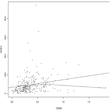
As a simple illustration of modern statistical tech-niques, we consider the association between awaken-ing cortisol and DHEA in older adults, again usawaken-ing the Well Elderly data. As previously indicated, there are outliers associated with both variables, but to il-lustrate some technical issues, outliers are momentar-ily retained. Then Pearson’s correlation is r = .136 with p = .031 (based on Student’s t) indicating that there is an association. From basic training, this result suggests that as cortisol increases, so does the expected value of DHEA. If, however, one uses the HC4 method for dealing with heteroscedasticity (via the R function pcorhc4), p = .49. Moreover, a test of the hypothe-sis that there is homoscedasticity (using the R func-tion qhomt) rejects (p = .016), the main point being that a homoscedastic method can give a substantially different result compared to one designed to deal with heterocedasticity. (The reverse also happens where a heteroscedastic method is highly significant but a ho-moscedastic method is not.)
A fairly obvious way of dealing with outliers is to use Spearman’s correlation, which is estimated to be
rs = .32 for the situation at hand, with p < .001
based on the usual Student’s t test, which assumes ho-moscedasticity. This result is fairly consistent with one reported in [1] wherers=.43,p=.003. Switching to a
heteroscedastic method (via the R function corb), again Spearman’s correlation is significant (p < .001). Switch-ing to a skipped correlation, with the goal of takSwitch-ing into account the overall structure of the data when dealing with outliers, the correlation is now .23 suggesting that outliers are having some impact on Spearman’s corre-lation, but again a significant result is obtained using a heteroscedastic method (using the R function scorci,
p < .001 ).
is straight rejects (p < .001). Also, splitting the data in terms of whether cortisol is greater than or less than .4, the resulting regression lines have significantly different slopes. Now a positive association is found for cortisol less than .4 (using the R function regci), but no associ-ation is found when cortisol is greater than .4. So the general conclusion is that there is a positive association when cortisol is relatively low, but for higher levels of cortisol there is no indication of an association. Notice that Spearman’s correlation paints a decidedly differ-ent picture. It underestimates somewhat the strength of the association when cortisol is low and misleadingly suggests that there is positive association when cortisol is high.
Figure 5. Estimated regression line for predicting DHEA given cortisol using least squares and a smoother
In some situations, simply removing leverage points and using OLS gives very similar results to more mod-ern regression estimators. But caution is warranted be-cause outliers among the dependent variable can result in relatively poor power when using OLS. That is, a robust estimator is needed. The next two illustrations demonstrate both points.
First consider the association between a measure of meaningful activities and the cortisol awakening re-sponse (CAR), which is the change in cortisol measured at the time of awakening and again 30-60 minutes later, again using the Well Elderly data. Pruessner et al. [30] were the first to propose that the repeated assessment of the salivary cortisol increase after awakening might represent a useful and easily measured index of corti-sol regulation. Exhibiting an absence or an exacerba-tion of this increase is associated with several adverse psychological and physiological outcomes (e.g., [28, 29]. Meaningful activities were measured with the Meaning-ful Activity Participation Assessment (MAPA) instru-ment, which was studied [9] and found to be a reliable and valid measure of meaningful activity, incorporating both subjective and objective indicators of activity en-gagement. For the version of MAPA used here, higher scores reflect a greater activity participation, with an individual’s MAPA score consisting of the sum of 29, 7-point Likert scales. The range of observed scores was 0-97 with 14 outliers based on the MAD-median rule.
Applying OLS with the usual Student’s t test, no asso-ciation is found (p=.88), and a heteroscedastic method fails to reject as well (p=.96). But removing leverage points (using a MAD-median rule), now a significant re-sult is obtain (p=.005). Using the Theil–Sen estimator,
p=.08 when leverage points are retained andp=.007 when leverage points are removed. So even when using a modern regression estimator, it can be important to check the impact of removing leverage points.
[image:8.595.321.515.337.530.2]To illustrate the potential impact of outliers among the dependent variable, consider the goal of predicting the CAR given a MAPA score. Using a smoother in a manner that deals with outliers yields the solid line shown in Figure 6. The nearly identical dashed line is the Theil–Sen regression line. The nearly horizontal (dotted) line is the least squares regression line. Us-ing the usual Student’s t test in conjunction with the least squares regression line yields a nonsignificant re-sult (p=.80) and removing leverage points again yields a nonsignificant result (p=.94). But using the Theil– Sen estimator, p =.033, and when leverage points are removed,p=.023.
Figure 6. Regression lines for predicting MAPA given CAR. The nearly horizontal line is the least squares regression line.
depressive symptoms into account.
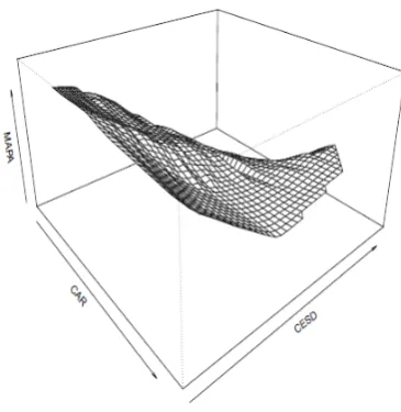
[image:9.595.87.270.224.412.2]However, look at Figure 7 which shows a smooth for predicting MAPA given CESD and the CAR. Note that there appears to be a distinct bend where the CAR is approximately 18. That is, there appears to be curva-ture with the nacurva-ture of the association changing when depressive symptoms are relatively high. Using only the data where CAR is less than 18, now the slope associated with CAR is significant (p=.043). Also, a significant difference was obtained between the slope for CAR less than 18 compared to when CAR is greater than or equal to 18 (p=.027).
Figure 7. The regression surface for predicting MAPA given CAR and CESD
7
Conclusions
Generally, robust methods are aimed at characteriz-ing the typical response. When distributions are skewed, the 20% trimmed mean and M-estimators tend to have values close to the median. In contrast, the mean can be highly atypical. However, situations arise where com-paring the tails of distributions can be important. For example, in the Well Elderly study, one goal was to com-pare the intervention group to a control in terms of de-pressive symptoms. But the bulk of the participants had relatively low CESD scores prior to intervention, suggesting that for the typical person there would be lit-tle improvement after intervention. Comparing medians found no significant difference, but a plot of the distri-butions indicated that differences in the right tails might exist. Indeed, comparing the upper quantiles yielded a significant difference. More precisely, among the more depressed individuals, intervention was found to be ben-eficial [45].
When considering the many new methods that have been derived, there is a seemingly natural question. Which method is best? But based on current technology, there is perhaps a better question: How many methods does it take to understand how groups compare or the association among the variables of interest? Different methods are sensitive to different features of the data and can provide different perspectives that have clinical
importance. The method that maximizes power is un-known. But a strategy that is clearly unsatisfactory is to use classic methods for means and assume all is well. Standard rank-based methods reduce problems associ-ated with outliers, but again more modern techniques have practical advantages.
Although the optimal regression method cannot be de-termined with certainty, there are some broad strategies that might be used. First, take advantage of smoothers. And when comparing groups, it can be helpful to plot estimates of the distributions. (The R functions akerd and g2plot are two good choices, which use kernel den-sity estimators.) As was illustrated, checks for curvature can be crucial. Second, do not assume that testing as-sumptions justifies methods that assume normality or homoscedasticity. All indications are that generally, the safest way of knowing whether a more modern method makes a practical difference is to actually try it. There is, however, the issue of multiplicity: controlling the the probability of one or more Type I errors when multiple tests are performed. One possibility is to choose some robust method for general use and if it fails to reject, consider an exploratory study where other techniques are used to analyze the data. One could then perform a confirmatory study. This, of course, would take some effort, but simultaneously it is important to not miss strong associations among the bulk of the data due to the statistical method that was used. Another strategy is to use a few well chosen techniques and control the probability of one or more Type I errors in some ap-propriate manner. For example, use some modern im-provement on the Bonferroni method such as the method derived by Rom [34].
Finally, it is not being suggested that least squares methods be abandoned. It is being suggested, however, that heteroscedastic methods are generally superior to homoscedastic methods and that checks on the impact of removing leverage points can be highly valuable. Also, robust regression estimators and smoothers deserve se-rious consideration. We have the technology for get-ting a deeper and more accurate understanding of data. Software for applying these methods is readily available. All that remains is taking advantage of modern methods when analyzing data.
REFERENCES
[1] Boudarene M., Legros, J. J., & Timsit-Berthier, M. (2002). DHEAs were dependent on cor-tisol, as shown by the close correlation be-tween both hormones. Encephale, 28, 139–146. http://www.ncbi.nlm.nih.gov/pubmed/11972140
[2] Brunner, E., Domhof, S. & Langer, F. (2002). Non-parametric Analysis of Longitudinal Data in Factorial Experiments. New York: Wiley.
[4] Cleveland, W.S., Devlin, S.J., 1988. Locally-weighted Regression: An Approach to Regression Analysis by Local Fitting. Journal of the American Statistical Association, 83, 596–610.
[5] Cliff, N. (1996). Ordinal Methods for Behavioral Data Analysis. Mahwah, NJ: Erlbaum.
[6] Cressie, N. A. C. & Whitford, H. J. (1986). How to use the two sample t-test. Biometrical Journal, 28, 131–148.
[7] Cribari-Neto, F. (2004). Asymptotic inference under heteroscedasticity of unknown form. Computational Statistics & Data Analysis, 45, 215–233.
[8] Doksum, K. A., Wong, C.-W., 1983. Statistical tests based on transformed data. Journal of the American Statistical Association, 78, 411–417.
[9] Eakman AM, Carlson ME, Clark, FA. (2010). The meaningful activity participation assessment: a mea-sure of engagement in personally valued activities Int J Aging Hum Dev., 70, 299–317.
[10] Efromovich, S., 1999. Nonparametric Curve Estima-tion: Methods, Theory and Applications. New York: Springer-Verlag.
[11] Eubank, R. L., 1999. Nonparametric Regression and Spline Smoothing. New York: Marcel Dekker.
[12] Foley K., Reed P., Mutran E., et al., 2002. Measurement adequacy of the CES-D among a sample of older African Americans. Psychiat Res, 109, 61–9.
[13] Fox, J. 2001. Multiple and Generalized Nonparametric Regression. Thousands Oaks, CA: Sage.
[14] Fung, K. Y. (1980). Small sample behaviour of some nonparametric multi-sample location tests in the pres-ence of dispersion differpres-ences. Statistica Neerlandica, 34, 189–196.
[15] Ghiciuc CM, Cozma-Dima CL, Pasquali V, Renzi P, Simeoni S, Lupusoru CE, Patacchiol, FR. Awakening responses and diurnal fluctuations of salivary cortisol, DHEA-S and sAA in healthy male subjects. Neuroen-docrinol Lett. 2011; 32: 475–480.
[16] Godfrey, L. G. (2006). Tests for regression models with heteroskedasticity of unknown form. Computational Statistics & Data Analysis, 50, 2715–2733.
[17] Gy¨orfi, L., Kohler, M., Krzyzk, A. Walk, H., 2002. A Distribution-Free Theory of Nonparametric Regression. New York: Springer Verlag.
[18] Hampel, F. R., Ronchetti, E. M., Rousseeuw, P. J. Sta-hel, W. A., 1986. Robust Statistics. New York: Wiley.
[19] Hand, A. (1998). A History of Mathematical Statistics from 1750 to 1930 New York: Wiley.
[20] H¨ardle, W., 1990. Applied Nonparametric Regression. Econometric Society Monographs No. 19, Cambridge, UK: Cambridge University Press.
[21] Heritier, S., Cantoni, E, Copt, S. Victoria-Feser, M.-P., 2009. Robust Methods in Biostatistics. New York: Wiley.
[22] Huber, P. J. & Ronchetti, E. (2009). Robust Statistics, 2nd Ed. New York: Wiley.
[23] Jackson, J., Mandel, D., Blanchard, J., Carlson, M., Cherry, B., Azen, S., Chou, C.-P., Jordan-Marsh, M., Forman, T., White, B., Granger, D., Knight, B., Clark, F. , 2009. Confronting challenges in intervention re-search with ethnically diverse older adults: the USC Well Elderly II trial. Clinical Trials, 6, 90–101.
[24] Lewinsohn, P.M., Hoberman, H. M., Rosenbaum M., 1988. A prospective study of risk factors for unipolar depression. J Abnorm Psychol, 97, 251–64.
[25] Maronna, R. A., Martin, D. R. & Yohai, V. J. (2006). Robust Statistics: Theory and Methods. New York: Wiley.
[26] Ng, M., Wilcox, R. R., 2011. A comparison of two-stage procedures for testing least-squares coefficients under heteroscedasticity. Brit J Math Stat Psych, 64, 244– 258.
[27] Pernet, C. R., Wilcox, R., Rousselet, G A. (2013). Ro-bust correlation analyses: a Matlab toolbox for psychol-ogy research. Fontiers in Psycholpsychol-ogy, January, Methods Article. doi: 10.3389/fpsyg.2012.00606
[28] Portella, M. J., Harmer, C. J., FLint, J., Cowen, P. and Goodwin, G. M., 2005. Enhanced early morning salivary cortisol in neuroticism. Amer J Psychiatry, 162, 807–809.
[29] Pruessner, J. C., Hellhammer, D. H., Kirschbaum, C., 1999. Burnout, perceived stress, and cortisol responses to awakening. Psychosomatic Med, 61, 197–204.
[30] Pruessner, J. C., Wolf, O. T., Hellhammer, D. H., Buske-Kirschbaum, A. B., von Auer, K., Jobst, S., Kirschbaum, C., 1997. Free cortisol levels after awak-ening: A reliable biological marker for the assessment of adrenocortical activity. Life Sci, 61, 2539–2549.
[31] R Development Core Team, 2010. R: A language and environment for statistical computing. R Foundation for Statistical Computing, Vienna, Austria. ISBN 3-900051-07-0, URL http://www.R-project.org.
[32] Radloff, L., 1977. The CES-D scale: a self report de-pression scale for research in the general population. Appl Psych Meas 1, 385–401.
[33] Rasmussen, J. L., 1989. Data transformation, Type I error rate and power. Brit J Math Stat Psych, 42, 203– 211.
[34] Rom, D. M., 1990. A sequentially rejective test pro-cedure based on a modified Bonferroni inequality. Biometrika, 77, 663–666.
[35] Rosenberger, J. L. & Gasko, M. (1983). Comparing location estimators: Trimmed means, medians, and trimean. In D. Hoaglin, F. Mosteller and J. Tukey (Eds.) Understanding Robust and exploratory data analysis. (pp. 297–336). New York: Wiley.
[36] Rousseeuw, P. J., Leroy, A. M., 1987. Robust Regression & Outlier Detection. New York: Wiley.
[38] Staudte, R. G., Sheather, S. J. (1990). Robust Estima-tion and Testing. New York: Wiley.
[39] Theil, H. (1950). A rank-invariant method of linear and polynomial regression analysis. Indagationes Mathe-maticae, 12, 85–91.
[40] Tukey, J. W. & McLaughlin D. H. (1963). Less vulner-able confidence and significance procedures for location based on a single sample: Trimming/Winsorization 1. Sankhya A, 25, 331–352.
[41] Westfall, P. H. & Young, S. S. (1993). Resampling Based Multiple Testing New York: Wiley.
[42] Wilcox, R. R. (2012). Modern Statistics for the Social and Behavioral Sciences: A Practical Introduction. New York: Chapman & Hall/CRC press
[43] Wilcox, R. R. (2012). Introduction to Robust Estima-tion and Hypothesis Testing 3rd EdiEstima-tion. San Diego, CA: Academic Press.
[44] Wilcox, R. R. & Clark, F. (in press). Robust regres-sion estimators when there are tied values. Journal of Modern and Applied Statistical Methods.
[45] Wilcox, R. R., Erceg-Hurn, D., Clark, F. & Carlson, M. (2013). Comparing two independent groups via the lower and upper quantiles. Jour-nal of Statistical Computation and Simulation. DOI: 10.1080/00949655.2012.754026
[46] Wolf , J. M., Nicholls, E. Chen, E. (2008). Chronic stress, salivary cortisol, and alpha-amylase in children with asthma and healthy children. Biological Psychol-ogy, 78, 20–28.
[47] Yohai, V. J. (1987). High breakdown point and high effi-ciency robust estimates for regression. Annals of Statis-tics, 15, 642–656.