A FRAMEWORK FOR ARABIC SENTIMENT ANALYSIS USING MACHINE LEARNING CLASSIFIERS

4519

A DETAILED ANALYSIS OF NEW INTRUSION DETECTION

DATASET

1_{MOHAMMED HAMID ABDULRAHEEM,} 2_{NAJLA BADIE IBRAHEEM}

1_{Department of Computer Sciences, University of Mosul, Iraq} 2_{Department of Computer Sciences, University of Mosul, Iraq}

E-mail: 1_{[email protected],} 2_{[email protected]}

ABSTRACT

The increasing use of Internet networks has led to increased threats and new attacks day after day. In order to detect anomaly or misused detection, Intrusion Detection System (IDS) has been proposed as an important component of secure network. Because of their model free properties that enable them to identify the network pattern and discover whether they are normal or malicious, Machine-learning technique has been useful in the area of intrusion detection. Different types of machine learning models were leveraged in anomaly-based IDS. There is an increasing demand for reliable and real-world attacks dataset among the research community. In this paper, a detailed analysis of most-recent dataset CICIDS2017 has been made. During the analysis, many problems and shortcoming in a dataset were found. Some solutions are proposed to fix these problems and produce optimized CICIDS2017 dataset. A 36-feature has been extracted during the analysis, and compared to 23-featured extracted by the dataset from literatures. The 36-features gave the best result of losses, accuracy and F1-score metrics for the testing model.

Keywords: CICIDS2017, Network Anomaly Detection, Imbalance Dataset, Quantile Transform, Machine Learning.

1. INTRODUCTION

Network security is becoming increasingly important with the rising growth of computer networks and the vast growing use of computer applications on these networks. All computer systems suffer from security gaps. It becomes difficult in practice and economically costly to solve these gaps by manufacturers. The role of intrusion detection systems in detecting anomalies and attacks in the network has become very important.

The use of intrusion detection systems is very important in research because it has the ability to detect new attacks while misuse detection systems are used in commercial applications. Several methods use machine intelligence methods in intrusion detection systems, few of them are based on the methods of detecting anomalies. To discover the percentage and decrease in this area, a lot of researches have been accomplished in this field and found that the datasets used contain potential problems.

Current Anomaly Intrusion detection methods are suffering from accurate performance. This is because no reliable tested are conducted and datasets are not verified. Since 1998 until now eleven datasets have appeared. Some of these datasets suffer from providing diversity and volume of network traffic, some do not contain different or latest attack patterns, while others lack feature set metadata information. Hence, there is a need for comprehensive framework for generating intrusion detection system benchmarking dataset. In 2016 Gharib et al., [1] have identified 11 criteria that are important for building a reliable dataset. None of the existing (intrusion detection system) datasets could cover all the 11 criteria. The 11 criteria of this framework are "complete network configuration, complete traffic, labeled dataset, complete interaction, complete capture, available protocols, attack diversity, anonymity, heterogeneity, feature set and metadata". Researchers at Canadian Institute of Cyber security have shown that most datasets are out of date and unreliable for evaluation purposes [2].

4520 Researchers at Canadian Institute of Cyber security provide this dataset. It contains up-to-date attacks and fulfills all the criteria of IDS that mentioned above. The dataset consists of CSV files for flow records generated with CICFlowMeter, and the sniffed network traffic PCAP files. Traffic Data captured for a total of five days. Attacks carried out on working days (Tuesday-Friday) in both morning and afternoon. The implemented attacks include DoS, DDoS, Heartbleed, Web Attacks, FTP Brute Force, SSH Brute Force, Infiltration, Botnet and Port Scans. Monday is the normal day and includes only legitimate traffic [3].

The CICIDS2017 Dataset builds from an abstract behavior of 25 internet users, which are based on email protocols and the HTTP HTTPS FTP SSH. It involves labeled network flows comprising full packet payloads in PCAP format, the corresponding

profiles and the labeled flows

(GeneratedLabelledFlows.zip), and CSV files for deep learning purpose (MachineLearningCSV.zip) are accessible [4]. Table 1 [5] shows the description of CICIDS2017 dataset.

The CICIDS 2017 is a new intrusion dataset, and not been studied well, so it is likely to contain mistakes and shortcomings. In this research we are trying to ask questions against the dataset, these questions contribute to optimized and prepare the dataset to be ready for consuming by machine learning algorithms. Consequently, it contributes to a high detection rate of the intrusion detection system for all attacks in the data set. The following questions will be the search path:

Is the dataset contains null values? Null values not accepted by Machine Learning algorithms. What type of values of the features in the data set? The suitability of those values for Machine Learning algorithms.

Are there any high correlations between the features in the data set? Highly correlations mean redundant features.

What is the important value of the features for classifying given attacks? Some features may have no effect in the detection of the given attacks.

Is the data set balanced, and what is the best method for balancing the dataset? Imbalanced

dataset makes the machine learning algorithm bias to large instances for a given attack. What is the suitable normalization function that results in the best detection rate? Not all normalization functions are suitable for all data set.

Table 1: CICIDS2017 dataset [5]

Flow Record ing Day (Worki ng Hours) pcap File size Duration CS V File Size

Attack name Flow

count

M

onday

10 GB

All Day 257 MB

No Attack 529918

T

uesday

10

GB All Day 166 MB FTP-Patator, SSH-Patator 445909

Wednesday

12 GB

All Day 272 MB Dos Hulk, DosGoldenEye, DOSslowloris, DosSlowhttptest, Heartbleed 692703 T hur sday 7.7

GB Morning 87.7 MB Web Attacks (Brute Force, XSS, Sql Injection) 170366 Afternoo n 103 MB

Infiltration 288602

Friday

8.2 GB

Morning 71.8 MB

Bot 192033

Afternoo n

92.7 MB

DDoS 225745

Afternoo n

97.1 MB

Port Scan 286467

4521 solutions to inherent shortcomings in this dataset and relabeling it to reduce high-class imbalance. Hossen et al. [4] explored the performance of a Network Intrusion Detection System (NIDS) that can detect various types of attacks in the network using Deep Reinforcement Learning Algorithm, they worked on 85 attributes of CICIDS2017 which aided as an effective means in the detection of different types of attacks. Kostas [5] tried to detect network anomaly by using machine-learning algorithms, the CICIDS2017 is used due to its up-to date, and has wide attack diversity. Feature selection made by using the Random Forest Regressor algorithm. Seven Different machine-learning methods are used in the implementation step and achieved high performance. Boukhamla et al. [7] described optimized CICIDS2017 dataset, and then evaluated the performance by using machine-learning algorithms. Again, the study used CSV file, which contains features obtained from network flow. Mieden [8] presented many experiments on classifying unwanted behavior in CICIDS2017 dataset using deep learning with tensor flow. They worked on CSV files which contains 85 features. Pektas et al. [9] presented deep learning architecture combining CNN and LSTM to enhance the intrusion detection performance. The CICIDS2017 dataset is used for testing the model. Vijayanand et al. [10] proposed IDS that used the genetic algorithm as a feature selection method and multiple Support Vector Machines (SVM) for classification. A small portion of the CICIDS2017 dataset instances are used to evaluate the system. Radford et al. [11] compared and contrasted a frequency-based model from five sequence of aggregation rules with sequence-based modeling of the Long Short-Term Memory (LSTM) recurrent neural network. Lavrova et al. [12] analyzed the CICIDS2017 dataset using digital wavelets. Watson [13] applied the Multi-Layer Perceptron (MLP) classifier algorithm and a Convolutional Neural Network (CNN) classifier that used the Packet Capture file of CICIDS2017. They selected specified network packet header features for their study. Aksu et al. [14] proposed a denial of service IDS that used the Fisher Score algorithm for features selection and Support Vector Machine (SVM), K-Nearest Neighbor (KNN) and Decision Tree (DT) as the classification algorithm. Marir et al. [15] use a distributed Deep Belief Network (DBN) as the dimensionality reduction approach. The obtained features are fed to a multi-layer ensemble SVM. The researchers divided CICIDS2017 dataset into training and test datasets using a ratio of 60% to 40%, respectively. Bansal

[16] proposed a data dimensionality reduction method for network intrusion detection. The model has been evaluated on both the datasets NSL-KDD and CICIDS 2017. And the comparison between both the proposed approaches has also been represented.

The CICIDS2017 dataset consists of two zipped files: GeneratedLabelledFlows and MachineLearningCVE. the first file consists of 85 features plus one for attacks type labels, while the second file consist of 78 features plus one for attacks type labels. The difference between the features in the files is 6 features these features in the first file is for identification the flow as stated by the authors of the dataset. All previous works on CICIDS2017 dataset except [3] used all 85 features of data. Some of these features such as “FlowID, SourceIP, SourcePort, DestinationIP” in the first file wrongly considered as a features to train the model. For example, the IP addresses and the source ports are changing continuously throughout the network. Inaddition the FlowID consist of 4 tuple they are “SourceIP, SourcePort, DestinationIP, DestinationPort” is considered a repeated feature. Therefore we used the second file for analysis and training. For the imbalance problem, the study [6] solve class imbalance problem by relabeling of classes. They merged a few minority class to form new attack classes (DoS and DDoS merged in one class, all Web attacks merged in one class too), the merging process incorrect. According to our result, DoS attack and DDoS attacks can be discriminated clearly. For dataset normalization, all of the previous literature used MiniMax or Standard scaling function. Our work use Quintile transform which give us better results.

4522 function of the data. We evaluated the performance of the optimized dataset by using machine-learning algorithm multilayer perceptron (MLP). The rest of this paper is organized as follows: Section 2 presents the analysis solutions and optimization of dataset in two stages. First, the solutions to clean up and remove shortcoming in the dataset are presented followed by analysis stage to select the best features and produce optimized dataset. Section 3 shows the model setting and metrics used to measure Performance of the new featured dataset using MLP machine-learning algorithm . Section 4 presents the results and discussion and finally section 5 shows the conclusions.

2. ANALYSIS AND OPTIMIZATION OF CICIDS2017 DATASET

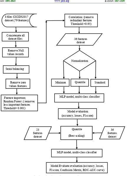
The Hardwar and software tools used in this research are CPU: Intel ® Core ™ i5-2450M CPU @ 2.5 GHz, RAM 8 GB OS: Windows 10 64-bit, Programming Language: Python. Libraries used: python package for scientific computing Numpy [17], machine-learning library Scikit-learn [18], Python Data Analysis Library Pandas [19], Python Deep Learning library Keras and Tensor flow [20], and python dataset balancing library IMBLEARN [21], Figure 1 shows overall process during this research.

2.1 Preparing the Dataset for Machine Learning

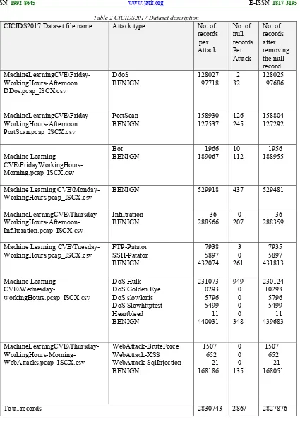
The machine learning file of the CICIDS2017 dataset (MachineLearningCSV.zip) downloaded from [2], the zipped file contains eight CSV files that represent the profile of the network traffic for five days, which includes normal and attack traffic for each day. After reading all the files in the analysis environment using Pandas, the details of the normal and attack traffic records for each File are shown in Table 2. The dataset shape in terms of the number of records and number of features was as follows, 2830743 rows, 78 feature Columns, 1 label Column.

Referring to Table 2, it is noted that the data set contains a number of records with null values. Machine learning algorithms do not consume null values. Since these values represent a small percentage of the number of records associated with each attack. Therefore, we delete those records from the data set.

The following Pandas library commands illustrate the operation of reading, viewing and cleaning one of the eight files:

Read the file in a Bot dataframe:

import pandas as pd Bot=pd.read_csv

("F:\MachineLearningCVE\Friday-WorkingHours-Morning.pcap_ISCX.csv")

The following command view information about columns in the Bot data farm:

Bot.info ()

Part of the output is shown in Table 3. We notice the file contain 79 columns the label column is an object type and the rest is of the numerical, float or integer. The numbers of records are 191033. The

following command counts the label column values:

Bot['Label'].value_counts()

Output:

BENIGN 189067 Bot 1966

The file contains 189067 record of BENIGN label and 1966 records of Bot label. To search for columns of Null values in the Bot data frame, we run the command:

null_columns=Bot.columns[Bot.isnull().any()] Bot[null_columns].isnull().sum()

Output:

FlowBytesPs 122 FlowPacketsPs 122 dtype: int64

The file has two columns FlowBytesPs and FlowPacketsPs with 122 values of Null in each. To see if the null values are in the witch label record we run the command:

Nullvalues=Bot[Bot.isnull().any(1)] Nullvalues['Label'].value_counts()

Output:

BENIGN 112 Bot 10

4523 have null values with label of Bot. To delete any record have a Null values we run the command:

Bot=Bot.dropna(axis=0, how='any')

The same operations are applied to all files. Then we merge all files to form a dataset for all attacks, by run the following commands:

AllAttacks=pd.concat([bot,ddos,dosH,infilt,ports ,ssh,web,benign],ignore_index=True)

Then the dataset shape becomes 2827876 rows, 78 feature Columns, 1 label Column. The distribution of records by traffic type in the data set shown in Table 4.

Table 4: Traffic flow type Distribution

Attack type Record

Count BENIGN DoS Hulk PortScan DdoS DoS GoldenEye FTP-Patator SSH-Patator DoS slowloris DoS Slowhttptest Bot

Web Attack-Brute Force Web Attack-XSS Infiltration Web Attack-Sql Injection Heartbleed 2271320 230124 158804 128025 10293 7935 5897 5796 5499 1956 1507 652 36 21 11

Total 2827876

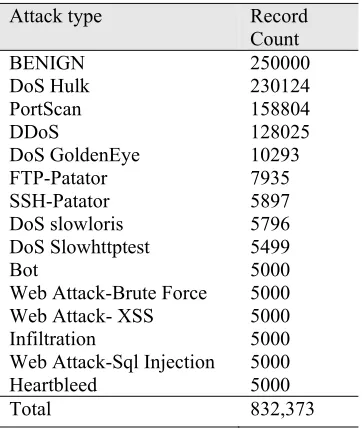
From Table 4, it is noted that the data set is imbalanced, as the number of normal traffic records is very large compared to other records of attacks, and the existence of a few records of some types of attacks. Many records for one class make the machine-learning model to bias to that class, while little records make the machine-learning model learn nothing about that class. To solve the problem of imbalance, the normal traffic records (BENIGN) is downsampled to 250000 records by using RandomUnderSampler a python algorithm in Imblearn balancing library. In addition, in order to increase the sensitivity of the classifier to detect attacks with few records in multi-class classification problems, the number of records for the few attacks (Bot Web Attack-Brute Force Web Attack-XSS Infiltration Web Attack-Sql Injection

Heartbleed) are increased so that minimum number of records of any attack type is not less than 5000 records. This is done using SMOTE (Synthetic Minority Over-sampling Technique), a python algorithm in Imblearn balancing library, which do upsample (generate new samples) from few records based on the n-nearest neighbor. The semi-balanced dataset becomes as shown in Table 5. After semi-balancing, the data set shape becomes as follows: 832,373 rows, 78 feature columns, 1 label Column.

Table 5: Semi-balanced dataset

Attack type Record

Count BENIGN DoS Hulk PortScan DDoS DoS GoldenEye FTP-Patator SSH-Patator DoS slowloris DoS Slowhttptest Bot

Web Attack-Brute Force Web Attack- XSS Infiltration Web Attack-Sql Injection Heartbleed 250000 230124 158804 128025 10293 7935 5897 5796 5499 5000 5000 5000 5000 5000 5000

Total 832,373

The following commands illustrate the process of downsampling. We import the balancing library then define a dictionary with the number of records for each class:

from imblearn.under_sampling import RandomUnderSampler

Define a dictionary:

Down-Dic = {

'BENIGN' : 250000,

'DoS Hulk' : 230124,

'PortScan' : 158804,

'DDoS' : 128025,

'DoS GoldenEye' : 10293,

'FTP-Patator' : 7935,

'SSH-Patator' : 5897,

'DoS slowloris' : 5796,

'DoS Slowhttptest' : 5499,

'Bot' : 1956,

'Web Attack-Brute Force’:1507, 'Web Attack-XSS' : 652,

4524

'Web Attack-Sql Injection' :21,

'Heartbleed' : 11,}

We create an instance of the downsampler according to the defined dictionary above: DownSamp=RandomUnderSampler (sampling_strategy=Down-Dic, random_state=0) The labels are moved from the dataset in a separate list. Then the features data frame and the labels list become an input to the downsample. The output is a new feature data frame and new label list. AllAttacks,AllAttacks_lable=DownSamp.fit_ sample(AllAttacks,AllAttacks_lable) The upsampling is conducted in the same way, but the up sampler now is SMOTE and the dictionary is defend as follow: UP_DIC= { 'BENIGN' : 250000,

'DoS Hulk' : 230124,

'PortScan' : 158804,

'DDoS' : 128025,

'DoS GoldenEye' : 10293,

'FTP-Patator' : 7935,

'SSH-Patator' : 5897,

'DoS slowloris' : 5796,

'DoS Slowhttptest' : 5499,

'Bot' : 5000,

'Web Attack-Brute Force': 5000, 'Web Attack-XSS' : 5000,

'Infiltration' : 5000,

'Web Attack-Sql Injection' : 5000, 'Heartbleed' : 5000,}

2.2 Features Analysis

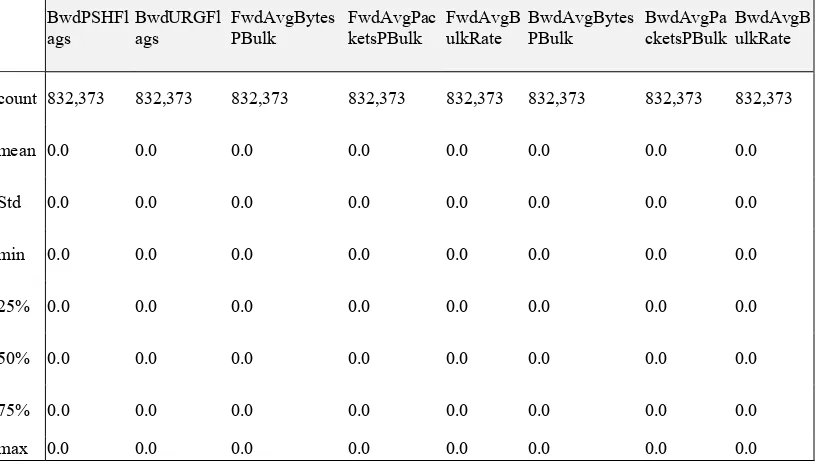
The data set contains 78 features in addition to one feature representing the traffic category (label). By viewing some basic statistical details of those data set features, 8 features were detected to have zero values, as shown in Table 6. That means those features have no effect on any calculation on the data set. Therefore, we removed them from the data set, the shape of the data set become 832,373 rows, 70 feature Columns, 1 label Column.

The values in Table 6 is obtained by following command: (that give us a statistical description about the dataset, such as maximum, minimum, standard deviation of each feature)

AllAttacks.Describe()

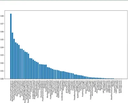
To analysis the remaining 70 features. we make feature reduction, two methods are used. The first is to find the importance of each feature in the dataset as a whole, through The Random Forest Algorithm. One of the main benefits of decision trees is interpretability. We can compare and visualize the relative importance of each feature. Features with splits that have a greater mean decrease in impurity. In scikit-learn machine learnning library, Random Forests can report the relative importance of each feature [22]. Wherethe algorithm gives the number between 0 and 1 for each feature and the total importance of all features is equal to 1, as shown in Figure 2.

The following commands illustrate the process to find feature importance by Random Forest classifier:

Load libraries.

From sklearn.ensemble import RandomForestClassifier

Create an instance of the classifier.

RF = RandomForestClassifier(random_state=0,

n_jobs=-1)

RFmodel=RF.fit(AllAttacks,AllAttacks_labl)

Calculate feature importances.

Importances=RFmodel.feature_importance_

The Importance variable is an array of the importance values of each feature in the data set. The following are some of the array values.

array([5.30263130e-02,

1.45516598e-02, 1.25230448e-02, 1.14137657e-02,2.57068785e-02, 2.35771754e-02, 1.87165275e-02, 4.19273221e-04,2.73702987e-02

,...,5.49352364e-04,8.77259231e-04, 2.03702912e-02, 5.41161681e-05])

4525 they are: (BwdIATMin, ActiveMax, URGFlagCount, ActiveMean, FwdPSHFlags,

FINFlagCount, SYNFlagCount,

BwdPacketLengthMin, IdleStd, FwdURGFlags, CWEFlagCount, ActiveStd, ECEFlagCount, RSTFlagCount ).

The dataset shape becomes as follows, 832,373 rows, 56 feature Columns, 1 label Column.

The second feature reduction method is to find the highly correlation between the features. Whenever the highly correlation between any two features is strong either directly or inversely, then one of them is considered redundant and preferably deleted. The correlation function [23] is used to find the correlation between the features. In addition, we put a threshold, if the correlation between two features is greater than (0.95) is considered highly correlation and one of the features should be removed. The Highly Correlated 20 Features (redundant) candidate to drop are: (TotalBackwardPackets,

TotalLengthofBwdPackets,

BwdPacketLengthMean, BwdPacketLengthStd, FwdIATTotal, FwdIATMax, FwdPacketsPs,

MaxPacketLength, PacketLengthStd,

AveragePacketSize, AvgFwdSegmentSize, AvgBwdSegmentSize, FwdHeaderLength, SubflowFwdPackets, SubflowFwdBytes, SubflowBwdPackets, SubflowBwdBytes, IdleMean, IdleMax, IdleMin).

The remaining 36 features are: (DestinationPort, FlowDuration, TotalFwdPackets, TotalLengthofFwdPackets, FwdPacketLengthMax, FwdPacketLengthMin, FwdPacketLengthMean, FwdPacketLengthStd, BwdPacketLengthMax, FlowBytesPs, FlowPacketsPs, FlowIATMean, FlowIATStd, FlowIATMax, FlowIATMin, FwdIATMean, FwdIATStd, FwdIATMin, BwdIATTotal, BwdIATMean, BwdIATStd,

BwdIATMax, FwdHeaderLength,

BwdHeaderLength, BwdPacketsPs,

MinPacketLength, PacketLengthMean, PacketLengthVariance, PSHFlagCount,

ACKFlagCount, DownPUpRatio,

InitWinBytesForward, InitWinBytesBackward, ActDataPktFwd, MinSegSizeForward, ActiveMin).

The data set shape became as follows, 832,373 rows, 36 feature Columns, 1 label Column.

3. MODEL SETTING AND METRICS USED TO MEASURE THE PERFORMANCE OF THE NEW OPTIMIZED DATASET

normalization is required for any dataset before applying any machine-learning algorithm we try three different normalization functions to choose the best one. In this, work, the process is done by Separation of data set into training data 70% and test data 30%. We try to use Three different normalization functions as follows:

a. Minimax or Unit Scaling:  The  aim  of  this  transformation  is  to  convert  the  range  of  a given feature into a scale that goes from  0  to  1.  Given  a  feature  f  with  a  range 

between  fmin  and  fmax  the 

transformation  is  given  by  equation  1  [24].

𝑓

b. Standard scaling (z-Score Scaling): An alternative method for scaling our features consists of taking into account how far away data points are from the mean. In order to provide a comparable measure, the transformation needed to carry out for a feature f with mean µf and standard deviation σf, is given by equation 2 [24].

c. Quantile scaling: A quantile refers to dividing a probability distribution into areas of equal probability. For example The median is a quantile; the median is positioned in a probability distribution so that precisely half of the data is lower than the median and half of the data is above the median. The median cuts a distribution into two equal areas and so it is referred to as 2-quantile. The median as the 0.5 quantile, with the ability that the percentage 0.5 (half) will be beneath the median and 0.5 will be above it. Equation 3 estimates the ith observation:

𝑖𝑡ℎ 𝑜𝑏𝑠𝑒𝑟𝑣𝑎𝑡𝑖𝑜𝑛 𝑞 𝑛 1 (3)

Where q is the quantile, n is the number of

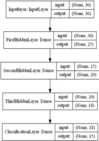
4526 To evaluate the performance of the three normalization functions, we used the dataset of 36 features and comparing the performance of a machine learning MLP model. The model is implemented in keras library; the structure of the model is shown in Figure 3.

Figure 3 the structure of the MPL model

The first layer is the input layer with nodes equal to the number of features in the dataset, followed by three dense layers with Relu activation function, and the final layer for classification of 15-class type with Softmax activation function corresponding to 15 categories of traffic types. The setting of hyper parameters for the model are: optimizer: Adam, Losses function: Categorical_Crossentropy, epochs: 70, batch_size: 128, number of class: 15, as shown in the Table 7.

Table 7: Classes name

Class No. Class Name class0 BENIGN class1 Bot

class2 DDoS

class3 DoS GoldenEye class4 DoS Hulk class5 DoS Slowhttptest class6 DoS slowloris class7 FTP-Patator class8 Heartbleed class9 Infiltration class10 PortScan

class11 SSH-Patator

class12 Web Attack-Brute Force class13 Web Attack-Sql Injection class14 Web Attack-XSS

The 3 normalization functions have been evaluated each with separate running of 70 epoch of the model, and then the best normalization function has been chosen based on the metrics below. Then the two datasets (36 features dataset, and 23 dataset features extracted by the authors in [3]) are evaluated using the best normalization function, each with separate running of the same model except the input layer to accommodate each feature number. The metrics used for evaluation multi-class classifier are:

a. Confutation matrix: For binary classifier the confusion matrix consist of four items they are, True Positives (TP): the classifier predict the true positive label as positive. True Negatives (TN): the classifier predicts the true negative label as negative. False Positives (FP): the classifier predicts the true negative label as positive. False Negatives (FN): the classifier predicts the true positive label as negative and arranged in a matrix as shown in Table 8.

Table 8: Confutation matrix

Confutation

matrix prediction

positive negative

Target

positive TP FN

negative FP TN

b. Accuracy Precision Recall and F1-Score: From the confusion matrix, the following Metrics can be computed corresponding to the equations 4,5,6,7 below [26]:

𝐴𝑐𝑐𝑢𝑟𝑎𝑐𝑦 (4)

𝑃𝑟𝑒𝑐𝑖𝑠𝑖𝑜𝑛 (5)

𝑅𝑒𝑐𝑎𝑙𝑙 (6)

4527 c. AUC - ROC curve: A receiver operating

characteristic curve (ROC) is a probability curve, and the area under the curve (AUC) represents degree or measure of separability. It is one of the most important evaluation metrics for testing the performance of any classification model at different threshold settings. It tells how much model is capable of distinguishing between classes. Higher the AUC better the model is at predicting 0s as 0s and 1s as 1s, see Figure 4 [28].

Figure 4: AUC - ROC curve

4. RESULTS AND DISCUSSION

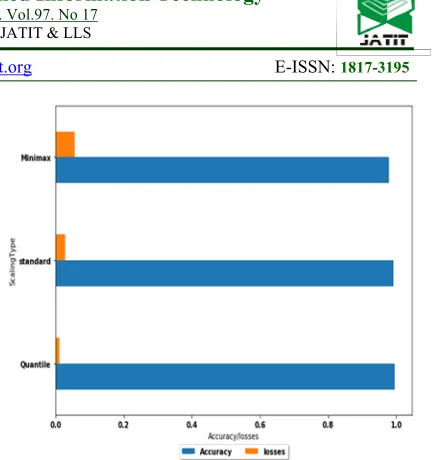
To find the best normalization function, the classifier model is run with the three different functions as mentioned above, and then the accuracy and losses of the classifier are computed as shown in Figure 5.

Figure 5: Scaling functions evaluation

In addition, F1-score of the classifier is computed with the three scaling functions, the result is shown in Figure 6.

According to the previous results, the Quantile scaling function gave better result than the two other functions, so it is the one used in our classifier.

The second step is to run the classifier model and evaluate a metrics according to the extracted 36 features dataset, and compare it to a 23- features dataset. The accuracy and losses of the classifier computed using our 36-features optimized data set and 23- features dataset, are summarized in Table 9.

Table 9: Accuracy and losses for the two dataset

No. of

features Accuracy losses

36 0.9927 0.0186

23 0.9886 0.0323

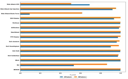
F1-score is computed for the classifier using two datasets, the results are shown in Figure 7.

4528 The confusion matrix for each class with regard to 36 features and 23 features is shown in Figure 8 and Figure 9 respectively. It is noticed that the majority of the Web Attack-XSS and Web Attack Brute-Force attacks samples are distributed between those two attacks, which indicates that those attacks have the same traffic properties, so they can be merged into one attack type.

The ROC- AUC curve for each class with 36 features and 23 features is shown in Figures 10 and 11 respectively, the average of AUC values of the 36 features dataset seemed to be slightly better than 23 features dataset.

5. CONCLUSIONS

There is an increasing demand for a reliable and real-world attacks dataset among research community. In this research, we investigated into a new intrusion dataset CICIDS2017. The analysis of the data set comprises of removing records of Null values, remove features with zero values, conduct a semi-balancing on the dataset to prevent biased to a large data and detect little records attacks. The features reduction process conducted by find the importance of the features in the dataset and removes less important features for classification and finds the high association between the features then removes the redundant features. The obtained result was a dataset of 36 features. To check this result we design an MLP model and split the dataset into training and test sets. At this point, the dataset needs to be normalized before feeding the model. We investigated for the best normalization function among MiniMax, standard, Quantile functions. To choose the best normalization function we training the MLP model 3 times each time using one normalizing function and compare the performance of the 3 classifiers on the test set and compute a classification metrics for each model, that comprise of accuracy, losses, F1-score, confusion matrix, and Roc-Auc curve. The best normalization function was the Quintile transform. Also, we compared the performance of the obtained 36 features dataset with a 23 features dataset, by training two MLP models (with the same preprocessing and the Quintile as a normalization function), one model on 36 features training set and the second on 23 features training set. Then we test the two models each one with its own tested set. Finally, we compute classification metrics for each model and compare it. From this research, we conclude the following results:

1. The CICIDS2017 dataset contains null values.

2. The CICIDS2017 dataset includes eight zero value features(BwdIATMin, ActiveMax, URGFlagCount, ActiveMean, FwdPSHFlags,

FINFlagCount, SYNFlagCount,

BwdPacketLengthMin, IdleStd,

FwdURGFlags, CWEFlagCount, ActiveStd, ECEFlagCount, RSTFlagCount ). The features in the dataset are obtained by CICFlowMeter packet capture application as stated by the author of the data set [3], it needs to be revised to see why the CICFlowMeter does not obtain the values of this features. These features may be significant to detect some attacks. This point never explored before.

3. The dataset includes redundant features detected with highly correlation function. The highly correlated features mean the features are redundant and contain the same information. Also the CICFlowMeter need to be tuned for redundant features.

4. The dataset includes less important features for classify any attack identified by random forest algorithm.

5. There is a trouble with the two attacks (Web Attack-Brute Force Web Attack-XSS) the most of the records of the two attacks classified as Web Attack-XSS, as clear in the confusion matrix of the two data sets, the trouble either came from the similarity between the two attacks or due to balancing algorithm. This point needs to be more investigated.

6. A Quantile scaling function is the best normalization function for this dataset, it gives the best metric values of the losses, accuracy, and F1-score compared to other scaling functions. We conclude that not all the data set is statistically the same. For each field of the data, there is more relevant normalization function for it. This point never explored before.

7. We extracted 36-feature, the 36-features gave the best result of losses, accuracy and F1-score metrics in the multi-class classifier MPL model compared to 23 features datasets.

4529 current work by implementing various balancing algorithm and investigate its effects on model learning. Study the trouble with the two attacks (Web Attack-Brute Force Web Attack-XSS). In addition, applying deep learning algorithms on this data set such as convolution and recurrent neural networks. At another direction a new dataset CSE-CIC-IDS2018 [2] dataset need to explored and analyzed. This dataset is huge and needs more hardware and computing resources to be analyzed.

REFRENCES:

[1] Gharib A, Sharafaldin I, Lashkari AH, Ghorbani AA., “An Evaluation Framework for Intrusion Detection Dataset”, International Conference on Information Science and Security (ICISS), 2016,1-6.

[2] Search UNB [Internet]. University of New Brunswick est.1785. [cited 2019May26].

Available from:

https://www.unb.ca/cic/datasets/ids-2017.html [3] Sharafaldin I, Lashkari AH, Ghorbani AA.,

“Toward Generating a New Intrusion Detection Dataset and Intrusion Traffic Characterization”, Proceedings of the 4th International Conference on Information Systems Security and Privacy, 2018, 108-116.

[4] Hossen, S., Janagam A., “Analysis of Network Intrusion Detection System with Machine Learning Algorithms (Deep Reinforcement Learning Algorithm)” [master’s thesis]. Karlskrona, Sweden: Faculty of Computing at Blekinge Institute of Technology; 2018. [5] Kostas, K., “Anomaly Detection in Networks

Using Machine Learning” [master’s thesis]. Colchester, UK: School of Computer Science and Electronic Engineering, University of Essex; 2018.

[6] Panigrahi R, Borah S., “A detailed analysis of CICIDS2017 dataset for designing Intrusion Detection Systems”, International Journal of Engineering & Technology 7 (3.24), 2018,

479-482.

[7] Boukhamla A, Gaviro JC., “CICIDS2017 dataset: performance improvements and validation as a robust intrusion detection system testbed” [pdf]. 2018 [cited

2019May26]. Available from:

https://www.researchgate.net/publication/3277 98156_CICIDS2017_Dataset_Performance_Im provements_and_Validation_as_a_Robust_Intr usion_Detection_System_Testbed

[8] Mieden, P., “Implementation and evaluation of secure and scalable anomaly-based network

intrusion detection” [bachelor thesis]. Munich: the Ludwig maximilians university, institute fur informatics; 2018.

[9] Pektaş A., Acarman T., “A deep learning method to detect network intrusion through flow‐based features”, International Journal of Network Management 29(3), 2018, e2050.

[10] Vijayanand R, Devaraj D, Kannapiran B., “Intrusion Detection System For Wireless Mesh Network Using Multiple Support Vector Machine Classifiers With Genetic-Algorithm-Based Feature Selection”, Computers & Security (77), 2018, 304–314.

[11] Radford BJ, Richardson BD, Davis SE., “Sequence Aggregation Rules for Anomaly Detection in Computer Network Traffic”, arXiv preprint arXiv: 1805.03735, 2018. [12] Lavrova D, Semyanov P, Shtyrkina A,

Zegzhda P., “Wavelet-Analysis Of Network Traffic Time-Series For Detection Of Attacks On Digital Production Infrastructure”, SHS Web of Conferences, EDP Sciences (44), 2018,

00052.

[13] Watson, G., “A Comparison of Header and Deep Packet Features When Detecting Network Intrusions”, Technical Report,

University of Maryland: College Park, MD, USA, 2018.

[14] Aksu D, Üstebay S, Aydin MA, Atmaca T., “Intrusion Detection With Comparative Analysis Of Supervised Learning Techniques And Fisher Score Feature Selection Algorithm”, International Symposium on Computer and Information Sciences , Springer,

Cham , 2018, 141-149.

[15] Marir N, Wang H, Feng G, Li B, Jia M. , “Distributed Abnormal Behavior Detection Approach Based On Deep Belief Network And Ensemble Svm Using Spark”, IEEE Access

(6),2018,59657-71.

[16] Bansal, A., “DDR Scheme and LSTM RNN Algorithm for Building an Efficient IDS”, [Master’s Thesis]. Punjab, India: Thapar Institute of Engineering and Technology; 2018.

[17] NumPy [Internet]. NumPy. [cited

2019May26]. Available from:

https://www.numpy.org/

[18] Learn [Internet]. scikit. [cited 2019May26]. Available from: https://scikit-learn.org/stable/

4530 [20] Keras: The Python Deep Learning library

[Internet]. Home - Keras Documentation. [Cited 2019May26]. Available from: https://keras.io/

[21] Lemaître G, Nogueira F, Aridas CK., “Imbalanced-learn: A Python Toolbox to Tackle the Curse of Imbalanced Datasets in Machine Learning”, The Journal of Machine Learning Research 18(1), 2017, 559-63.

[22] Albon, Chris. Machine Learning with Python Cookbook: Practical Solutions from Preprocessing to Deep Learning. OReilly

Media, 2018.

[23] pandas.DataFrame.corr [Internet]. pandas.DataFrame.corr - pandas 0.25.1 documentation. Available from:

https://pandas.pydata.org/pandas-docs/stable/reference/api/pandas.DataFrame.c orr.html

[24] Rogel-Salazar J., “Data Science and Analytics with Python”, Philadelphia, PA: Chapman and Hall/CRC, 2018,161-163

[25] Quantile: Definition and How to Find Them in Easy Steps [Internet]. Statistics How To. 2018 [cited 2019May26]. Available from: https://www.statisticshowto.datasciencecentral. com/quantile-definition-find-easy-steps/ [26] Kelleher JD, Namee BM, DArcy A.

Fundamentals Of Machine Learning For Predictive Data Analytics: Algorithms, Worked

Examples, And Case Studies. Cambridge

(Massachusetts): MIT Press, 2015.

[27] Understanding Categorical Cross-Entropy Loss, Binary Cross-Entropy Loss, Softmax Loss, Logistic Loss, Focal Loss and all those confusing names. [cited 2019May26].

Available from:

https://gombru.github.io/2018/05/23/cross_entr opy_loss/

[28] Narkhede S. Understanding AUC - ROC Curve [Internet]. Towards Data Science. Towards Data Science; 2018 [cited

2019May26]. Available from:

4531

Figure 1 Flowchart of Analysis and Optimization of CICIDS2017 Dataset

Concatenate all dataset files

 Remove zero values features

Feature important, Random Forest :( removes less important features Threshold< 0.001)

Semi-balancing Remove Null values records

MLP model, multi-class classifier Correlation: (remove

redundant features Threshold >0.95)

 Minimax 8 files CICIDS2017

dataset (79 features)

36 features dataset

Normalization

 Standard 

Quantile

 Model Evaluate evaluation (accuracy, losses, F1score, Confusion Matrix, ROC-AUC curve)

Model evaluation (accuracy, losses, F1score)

MLP model, multi-class classifier Quantile

(Best scaling) 23

features 

dataset

36 features

4532

Table 2 CICIDS2017 Dataset description

CICIDS2017 Dataset file name Attack type No. of records per Attack No. of null records Per Attack No. of records after removing the null record MachineLearningCVE\Friday-WorkingHours-Afternoon DDos.pcap_ISCX.csv DdoS BENIGN 128027 97718 2 32 128025 97686 MachineLearningCVE\Friday-WorkingHours-Afternoon PortScan.pcap_ISCX.csv PortScan BENIGN 158930 127537 126 245 158804 127292 Machine Learning CVE\FridayWorkingHours-Morning.pcap_ISCX.csv Bot

BENIGN 1966 189067 10 112 1956 188955

Machine Learning

CVE\Monday-WorkingHours.pcap_ISCX.csv BENIGN 529918 437 529481

MachineLearningCVE\Thursday- WorkingHours-Afternoon-Infilteration.pcap_ISCX.csv Infiltration BENIGN 36 288566 0 207 36 288359

Machine Learning CVE\Tuesday-WorkingHours.pcap_ISCX.csv FTP-Patator SSH-Patator BENIGN 7938 5897 432074 3 0 261 7935 5897 431813 Machine Learning CVE\Wednesday-workingHours.pcap_ISCX.csv DoS Hulk DoS Golden Eye DoS slowloris DoS Slowhttptest Heartbleed BENIGN 231073 10293 5796 5499 11 440031 949 0 0 0 0 348 230124 10293 5796 5499 11 439683 MachineLearningCVE\Thursday- WorkingHours-Morning-WebAttacks.pcap_ISCX.csv WebAttack-BruteForce WebAttack-XSS WebAttack-SqlInjection BENIGN 1507 652 21 168186 0 0 0 135 1507 652 21 168051

4533

Table 3 the output of the command Bot.info ()

Output

<class 'pandas.core.frame.DataFrame'> RangeIndex: 191033 entries, 0 to 191032 Data columns (total 79 columns):

DestinationPort 191033 non-null int64 FlowDuration 191033 non-null int64 TotalFwdPackets 191033 non-null int64 TotalBackwardPackets 191033 non-null int64 TotalLengthofFwdPackets 191033 non-null int64 TotalLengthofBwdPackets 191033 non-null int64 FwdPacketLengthMax 191033 non-null int64 FwdPacketLengthMin 191033 non-null int64 FwdPacketLengthMean 191033 non-null float64 FwdPacketLengthStd 191033 non-null float64 .

. . .

IdleMean 191033 non-null float64 IdleStd 191033 non-null float64 IdleMax 191033 non-null int64 IdleMin 191033 non-null int64 Label 191033 non-null object dtypes: float64(24), int64(54), object(1)

memory usage: 115.1+ MB

Table 6: Features with zero values

BwdPSHFl

ags BwdURGFlags FwdAvgBytesPBulk FwdAvgPacketsPBulk FwdAvgBulkRate BwdAvgBytesPBulk BwdAvgPacketsPBulk BwdAvgBulkRate

count 832,373 832,373 832,373 832,373 832,373 832,373 832,373 832,373

mean 0.0 0.0 0.0 0.0 0.0 0.0 0.0 0.0

Std 0.0 0.0 0.0 0.0 0.0 0.0 0.0 0.0

min 0.0 0.0 0.0 0.0 0.0 0.0 0.0 0.0

25% 0.0 0.0 0.0 0.0 0.0 0.0 0.0 0.0

50% 0.0 0.0 0.0 0.0 0.0 0.0 0.0 0.0

75% 0.0 0.0 0.0 0.0 0.0 0.0 0.0 0.0

4534

4535

Figure 6: F1-score of multi class classifier with different scaling functions

4536

Figure 8: Confusion matrix of 36 features

4537

Figure 10: AUC - ROC curve of 36 features

Figure 11: AUC - ROC curve of 23 features