Minimising Drop tail in the Network by Using Common Window together with Queue Mechanism

(1)

International Journal of Emerging Technology and Advanced Engineering

Website: www.ijetae.com (ISSN 2250-2459,ISO 9001:2008 Certified Journal, Volume 4, Issue 12, December 2014)

651

Minimising Drop tail in the Network by Using Common

Window together with Queue Mechanism

Harshit Nigam

1

, Akhilesh Singh

2

Dept of Computer Science and Engineering 1Lord Krishna College of Engineering Ghaziabad, 2United Institute of Technology Allahabad (U.P), India

Abstract—The algorithm for congestion control is the main reason we can use the Internet successfully today despite resource bottlenecks and largely unpredictable user access patterns. We use simulations to evaluate congestion control algorithms. NS-2 is used for the simulation. Effective resource utilization, such as bandwidth utilization, retransmission rate and window size, is compared. Our simulation results show that bias exists in both categories, so factors may affect the fairness are also simulated. We focus on the effect of different queue algorithms, such as Drop Tail and RED.

Keywords—Previous approach( Drop tail, Random Early Detection) , Modified Drop tail mechanism, Coding, Diagram And X graph.

I. INTRODUCTION

Bandwidth management is a way to control congestion. There are 2 algorithms used that are commonly utilized now days in network. Drop Tail and RED. Drop Tail is easy to implement but has problem of synchronization and RED is complicated but it avoid collision. Another way is:-QUEUE MANAGEMENT can also be used to control the queue size. It contains:- Passive Queue management:- Which drops packets when queue is full. Active queue management:-which drops packets before the buffer getting full.

II. DROP TAIL

Tail Drop, or Drop Tail, is a very simple queue management algorithm used by Internet routers, e.g. in the network schedulers, and network switches to decide when to drop packets. With tail drop, when the queue is filled to its maximum capacity, the newly arriving packets are dropped until the queue has enough room to accept incoming traffic as shown in figure 1. It uses First in first out algorithm.

Figure1: AN ILLUSTRATION OF DROP TAIL

III. RANDOM EARLY DETECTION

[image:1.612.326.561.239.316.2]

Random early detection (RED), also known as random early discard or random early drop is an queuing discipline for a network scheduler suited for congestion avoidance. If the buffer is almost empty, all incoming packets are accepted. As the queue grows, the probability for dropping an incoming packet grows too. When the buffer is full, then all incoming packets are dropped as shown in figure 2. It indirectly signal to sender and receiver by deleting some packets, if packets are deleted feedback is received late then sender start sending packets again eg:- when avg queue buffer length is more than max queue length threshold

[image:1.612.342.565.506.683.2]

(2)

International Journal of Emerging Technology and Advanced Engineering

652

IV. MODIFIED DROP TAIL MECHANISM

Modified Drop tail mechanism is a simple procedure as compared to Random Early Detection algorithm and over Drop tail which is very simple and not very effective. Here I used to compare both the method and generate the new one which is superior over the both and help to provide congestion control with in the network. I made two simulation method to test the performance of RED and Drop tail in wired network separately. But then I found the average packet losses are almost same in both the cases. Therefore while in communication if packets lost is there it will affect the Quality of services. Therefore to minimize it Modified Drop tail mechanism is used. As shown in Figure 3 and Figure 4.

V. CODING

set ns [new Simulator] # Open NAM trace file set nf [open out.nam w] $ns namtrace-all $nf # Open NS trace file set tf [open out.tr w] $ns trace-all $tf

# Open TCP cndw trace file set windowVsTime [open win w] # Open parameter recording file set param [open parameters w] # Define a 'finish' procedure proc finish {} {

global ns nf tf $ns flush-trace close $nf close $tf

exec grep "a" red-queue.tr > ave.tr exec grep "Q" red-queue.tr > cur.tr exec nam out.nam & exit 0

}

Under this section we will be creating the source node and destination nodes and providing the flow between them.

# Create bottleneck and dest nodes set n2 [$ns node]

set n3 [$ns node]

# Create RED links between bottleneck nodes $ns duplex-link $n2 $n3 0.7Mb 20ms RED # Set simulation parameters

set NumbSrc 3 set Duration 50

# Create $NumbSrc source nodes

for {set j 1} {$j<=$NumbSrc} { incr j } {

set S($j) [$ns node] }

# Create a random generator for starting the ftp and # for bottleneck link delays

set rng [new RNG] $rng seed 2

# parameters for random variables for begenning of ftp connections

set RVstart [new RandomVariable/Uniform] $RVstart set min_ 0

$RVstart set max_ 7 $RVstart use-rng $rng

# Define random starting times for each connection for {set i 1} {$i<=$NumbSrc} { incr i } { set startT($i) [expr [$RVstart value]] set dly($i) 1

puts $param "startT($i) $startT($i) sec" }

# Create links between source and bottleneck for {set j 1} {$j<=$NumbSrc} { incr j } {

$ns duplex-link $S($j) $n2 10Mb $dly($j)ms DropTail $ns queue-limit $S($j) $n2 20

} # Orient the links

$ns duplex-link-op $n2 $n3 orient right $ns duplex-link-op $S(1) $n2 orient right-down $ns duplex-link-op $S(2) $n2 orient right $ns duplex-link-op $S(3) $n2 orient right-up # Set Queue Size of (bottleneck) link (n2-n3) to 100 $ns queue-limit $n2 $n3 100

# Create TCP Sources

for {set j 1} {$j<=$NumbSrc} { incr j } { set tcp_src($j) [new Agent/TCP/Reno] $tcp_src($j) set window_ 8000 }

# Color the packets $tcp_src(1) set fid_ 1 $ns color 1 red $tcp_src(2) set fid_ 2 $ns color 2 yellow $tcp_src(3) set fid_ 3 $ns color 3 blue

# Create TCP Destinations

for {set j 1} {$j<=$NumbSrc} { incr j } { set tcp_snk($j) [new Agent/TCPSink] }

(3)

International Journal of Emerging Technology and Advanced Engineering

653

# Further parametrisation of TCP sources for {set j 1} {$j<=$NumbSrc} { incr j } { $tcp_src($j) set packetSize_ 552 }

# Create FTP sources

for {set j 1} {$j<=$NumbSrc} { incr j } { set ftp($j) [$tcp_src($j) attach-source FTP] }

# Schedule events for the FTP agents: for {set i 1} {$i<=$NumbSrc} { incr i } { $ns at $startT($i) "$ftp($i) start" $ns at $Duration "$ftp($i) stop" }

# plotWindow(tcpSource file k): Write CWND of k tcpSources in file

proc plotWindow {tcpSource file k} { global ns NumbSrc

set time 0.03 set now [$ns now]

set cwnd [$tcpSource set cwnd_]

if {$k == 1} {

puts -nonewline $file "$now \t $cwnd \t" } else {

if {$k < $NumbSrc } {

puts -nonewline $file "$cwnd \t" }

}

if { $k == $NumbSrc } {

puts -nonewline $file "$cwnd \n" }

$ns at [expr $now+$time] "plotWindow $tcpSource $file $k"

}

# Start plotWindow() for all tcp sources for {set j 1} {$j<=$NumbSrc} { incr j } {

$ns at 0.1 "plotWindow $tcp_src($j) $windowVsTime

$j" }

# Monitor avg queue length of RED link ($n2,$n3) in file "red-queue.tr"

set traceq [open red-queue.tr w] set redq [[$ns link $n2 $n3] queue] $redq trace curq_

$redq trace ave_

$redq attach $traceq # Schedule simulation end $ns at [expr $Duration] "finish" # run

$ns run

VI. DIAGRAM

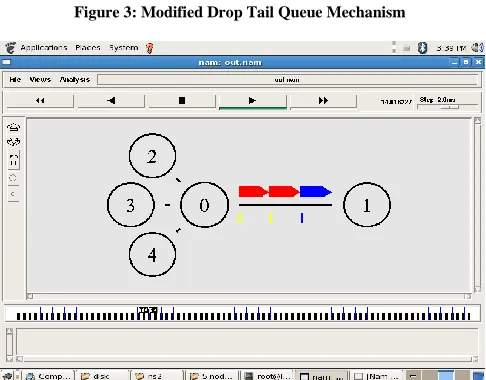
[image:3.612.325.571.276.442.2]

The diagram of the Modified Drop Tail queue is shown in the figure 3 and figure 4 . where dual links are used for communication between node 0-2, 0-3, 0-4, and the drop tail queue mechanism is used in node 0 and congestion window is used in node 2,3,4.

Figure 3: Modified Drop Tail Queue Mechanism

Figure 4: Modified Drop Tail Queue Mechanism

VII. X-GRAPH

[image:3.612.324.567.409.599.2]

(4)

International Journal of Emerging Technology and Advanced Engineering

654

[image:4.612.48.297.131.294.2]

The outcome or the result of the Modified Drop Tail Queue is shown in figure 5.

Figure 5: X graph Of Modified Drop Tail Queue Mechanism

VIII. CALCULATIONS

Let € be processing rate, T the period between calculations of discard probility and average occupancy , B the buffer size, and 0 < L < B the number of bytes in a buffer. Let us assume that all buffer consist of the same number of bytes L. the number of bytes L. The number of bytes R removed from the queue during the time T between consecutive calculations is:

R={ € * T / L}……….(i)

Where € is the rate of flow of packets per second from window , Rmax is the condition when no queue is used and

Rmin is the condition when queue size of 10 mb is used.

[image:4.612.51.286.538.660.2]

€ = 23.9 Mb/s , Rmax is obtained when L = 1 Mb while Rmin is reached when L= 10 Mb. As shown in Table 1.

Table 1:

Comparison between RED and Modified Algorithm

Period (T ) Rmax Rmin

1 Sec 23.90 Mb/s 2.39 Mb/s

2 Sec 47.8 0 Mb/s 4.78 Mb/s

5 Sec 119.50 Mb/s 11.95 Mb/s

10 Sec 239.00 Mb/s 23.90 Mb/s

As we can see the probability of discarding packet decreases when buffer is used together with RED algorithm as we can see that carrying capacity is only 10 mb between 2 nodes after that drop tail condition occurs.

IX. CONCLUSION

In this paper we evaluate Drop tail, Random Early Detection algorithm and Modified Drop tail mechanism, and found that in Modified Drop tail mechanism the loss is minimum as compare to both Drop tail, Random Early Detection algorithm and also common window was used to minimize the packet loss which can be adjusted according to the packet losses. Ultimately it can be used to for the communications on a network Link and to avoid network congestion and poor performance of the network

REFERENCES

[1] Z.Wang and J. Crowcroft. ―A new congestion control scheme: Slow

start and search (Tri-S).‖ Computer Rev Vol. 21. no.1, Jan. 1991, pp.32-43.

[2] T. Bonald, M. May, and J. C. Bolot. Analytic Evaluation of RED performance. IEEE INFOCOM 2000

[3] C.V. Hollot, V. Misra, D. Towsley and W. Gong, A control theoretic

analysis of RED, in: Proc. of INFOCOM’2001, April 2001, pp. 1510–1519.

[4] Schweitzer et al., 1993] Schweitzer,P.,Serazzi,G.,and

Broglia,M.(1993). A survey of bottleneck analysis in closed networks of queues.In Proceedings Performance Evaluation of

Computer and Communication Systems,pages 491-508,

Berlin,Germany. ACM.

[5] [Blake, 1979] Blake, R. (1979). Ta ilor: A simple model that works. In Proceedings Conference on Simulation, Measurement, and Modeling of Computer Systems, pages 111, Boulder, CO. ACM.

[6] [Blake, 1995] Blake, R. (1995). Optimizing Windows NT. Microsoft Press, Redmond, WA.

[7] [Breese et al., 1992] Breese, J., Horvitz, E., Peot, M.,Gay, R., and Quentin, G. (1992). Automated decision-analytic diagnosis of thermal performance in gas turbines. In Proceedings International GasTurbine And Aeroengine Congress and Exposition. American Society of Mechanical Engineers. 92-GT399.

[8] [Buzen, 1976] Buzen, J. (1976). Fundamental operational laws of computer system performance. Acta Informatica, 7: 167-182.

(5)

International Journal of Emerging Technology and Advanced Engineering

655 AUTHOR’S PROFILE

Harshit Nigam obtained Btech (HONOURS) in (Computer Science and Engineering) from G.B.T.U in 2011 and pursing Mtech (Computer Science) from United Institute of Technology Allahabad. He is working as a Assistant Professor in Lord Krishna college of Engineering Ghaziabad . His area of interest includes Information Security and Graph Theory. He has more than 3 years of experience.