TIME COMPLEXITY COMPARISON BETWEEN
AFFINITY PROPAGATION ALGORITHMS
1
R. REFIANTI, 2A.B. MUTIARA, 3S. GUNAWAN
1
Asst.Prof., Faculty of Computer Science and Information Technology, Gunadarma University, Indonesia
2
Prof., Faculty of Computer Science and Information Technology, Gunadarma University, Indonesia
3
Alumni, Graduate Program in Information System, Gunadarma University, Indonesia
E-mail: 1,2{rina,amutiara}@staff.gunadarma.ac.id
ABSTRACT
Affinity Propagation is one of clustering technique that use iterative message passing and consider all data points as potential exemplars. It is complimented because providing a good result of clustering with low error rate. But it has several drawback, such as quadratic computational cost and vague values of preference. There are many research trying to solve the drawback to improve the speed and quality of Affinity Propagation. But, there are not any test to find the best Affinity Propagation expansion algorithm in speed. This has led researchers to try to compare the performance of several Affinity Propagation expansion algorithms. The tested algorithms are Adaptive Affinity Propagation, Partition Affinity Propagation, Landmark Affinity Propagation, and K-AP. There are two comparison made in this paper: theoretical analysis and running test. From both comparison, it can be found that Landmark Affinity Propagation has the most efficient computational cost and the fastest running time, although its clustering result is very different in number of clusters than Affinity Propagation
Keywords: Affinity Propagation, Availability, Clustering, Exemplar, Responsibility, Similarity Matrix
1. INTRODUCTION
The world today contains an unimaginably vast amount of data which is getting even vaster ever more rapidly. According to [10], National Oceanic and Atmospheric Administration (NOAA) have a data center alone store more than 20 pentabytes, collects 80 TB of scientific data daily, and will increase ten-fold in 2020. Facebook, one of the biggest social-networking website, has a total of 40 billions photos [1]. With such big amount of data, the need of data processing along with the high processing speed is increasing along [17].
One of a way to obtain an information from a big amount of data is clustering analysis. Clustering is a process of partitioning a data set into several subsets unsupervisedly [8]. Clustering is one of a techniques in Knowledge Discovery on Data (KDD) or Data Mining which make subsets from the data set with the subset objects are similar to each other and dissimilar to objects in other subsets. Clustering is performed by clustering algorithm which is useful to find interesting group in a data. Clustering analysis has been widely implemented in different area, such as business intelligence, image
pattern recognition, Web search, biology, and security [8]. There are many clustering algorithm in literature, such as k-means, k-medoids, hierarchical clustering, etc.
make it faster by dealing with the drawback. Several approaches have been proposed to speed up the clustering. For example, Wang et al.’ s Adaptive AP, Xia et al.’ s Partition AP and Landmark AP, and Zhang et al.’ s K-AP. While all of those algorithms have shown a better performance in speed than the original Affinity Propagation, there are no comparation between those algorithm. This is what encourage researcher to compare those algorithm based on the performance.
2. LITERATURE REVIEW
2.1 Affinity Algorithm
Given a set of data points {x1,x2,x3,...,xn}, Affinity Propagation takes as input of similarity between data points { S }, where each similarity
] , [i j
s indicates how well data point xj is suited to
be an exemplar for xi. Any type of similarities is acceptable, e.g. negative Euclidean distance for real valued data and Jaccard coefficient for non-metricdata, thus Affinity Propagation is widely applicable in different areas.
Rather than requiring that the number of clusters be prespecified, Affinity Propagation takes as input a real number s[j,j] for each data point k so that data points with larger values of s[j,j] are more likely to be chosen as exemplars. These values are referred to as “ preferences.” These preferences will affect the number of clusters produced. The shared value could be the median of the input similarities (resulting in a moderate number of clusters) or their minimum (resulting in a small number of clusters).
Given similarity s[i,j]i,j=1,2,...,n , Affinity Propagation try to find the best exemplars that maximize the net similarity, i.e. the overall sum of similarities between all exemplars and their member data points. Process in Affinity Propagation can be viewed as passing values between data points. There are two values that are passed between data points: responsibility and availability. Resposbility
] , [i j
r is how well-suited point k is to serve as the exemplar for point i, taking into account other potential exemplars for point i. Availability a[i,j] reflects the accumulated evidence for how appropriate it would be for point i to choose point k as its exemplar, taking into account the support from other points that point k should be an exemplar.
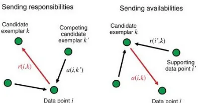
Fig.2.1. shows us how the responsbility and availability works in Affinity Propagation. Responsibilities r[i,j] are sent from data points to
[image:2.612.321.518.206.308.2]candidate exemplars and indicate how strongly each data point favors the candidate exemplar over other candidate exemplars. Availabilities a[i,j] are sent from candidate exemplars to data points to indicate the availability of candidate exemplars to data points as cluster point. All of this message passings are kept done until convergence is met or the iteration reach a certain number.
Figure 2.1. Message Passing in Affinity Propagation [4]
All responsibilities and availabilities are set to 0 initially, and their values are iteratively updated as follows to compute convergence values:
− ≠ + − ≠ ≠ ) = ( ]} , [ { ] , [ ) ( ]} , [ ] , [ { ] , [ = ] , [ j i k i s max j i s j i k i s k i a max j i s j i r j k j k (1)
+ ≠
∑
∑
≠ ≠ ) = ( ]} , [ {0, ) ( ]} , [ {0, ]} , [ {0, = ] , [ , j i j k r max j i j k r max j j r min j i a i k j i k (2)After calculating both responsibility and availability, their values are iteratively updated as follows to compute convergence values:
] , [ ] , [ ) (1 = ] ,
[i j ri j r i j
r −λ +λ ′
(3)
] , [ ] , [ ) (1 = ] ,
[i j ai j a i j
a −λ +λ ′
(4)
where λ is a damping factor introduced to avoid numerical oscillations, and r′[i,j] and a′[i,j] are previous values of responsbility and availability. λ should be larger than or equal to 0.5 and less than 1. High value of λ may make number oscillations avoided, but this is not guaranteed and a high value of λ will make the Affinity Propagation run slowly [9]. Upon convergence, a set of exemplar K is choosen by: ) 1,2,3,... = ]}( , [ ] , [ {
=argmax ri j ai j j N
[image:2.612.313.530.381.512.2]Affinity Propagation have several advantage over other clustering methods due to Affinity Propagation consideration of all data points as potential exemplars while most clustering methods find exemplars by keeping track of a fixed set of data points and iteratively refining it [4]. Because of it, most clustering methods does not change the set that much and just keep tracking on the particular sets. Furthermore, Affinity Propagation supports similarities that are not symmetric or do not satisfy the triangle inequality and it is not depend on initialization that found on other clustering algorithms. Because of these advantages, it has been successfully used in many applications in various diciplines such as image clustering [4] and chinese caligraphy clustering [20].
While Affinity Propagation has those advantages, it has a really big issue in speed especially for large scale datasets [23]. Affinity Propagation requires
) (N2T
O time to update the message where N and T
are respectively the number of data points and the number of iterations [5]. Due to this, researchs nowaday focus on this issue to improve the speed of it. We will review those research in the following sections.
2.2 Adaptive Affinity Propagation
Adaptive Affinity Propagation (Adaptive-AP) is designed to solve Affinity Propagation limitation : it is hard to know what value of parameter preference can yield an optimal clustering solution, and oscillations cannot be eliminated automatically if occur [18]. To solve the problem, Adaptive-AP can adapt to the need of the data sets by configuring the value of preferences and damping factor. Adaptive-AP capabilities including adaptive adjustment of the damping factor to eliminate oscillations (called adaptive damping), adaptive escaping oscillations by decreasing p when adaptive damping method fails (called adaptive escape), and adaptive searching the space of p to find out the optimal clustering solution suitable to a data set (called adaptive preference scanning).
Adaptive damping is a way to eliminate oscillations in cluster result. Adaptive damping works by checking whether oscillations occurs, increase λ by 0.05 if oscillations is detected, and iteratively doing it until the algorithms converge. But, oscillations’s features are too complex to be described [18]. But defining non-oscillation features is easier: the number of identified exemplars is decreasing or unchanging during the iterative process.
If increasing λ fails, in other words adaptive damping fails to decreasing the oscillations, adaptive escape is applied. Adaptive escape is designed as follows: when oscillations occur and
0.85
≥
λ in the iterative process, decreasing p gradually until oscillations disappear. Both of adaptive damping and adaptive escape are designed to works together, the procedures are shown on Algorithm 1.
Algorithm 1. Adaptive Damping and Adaptive
Escape
1. Initializeλ=0.5, monitoring window size w =
40, w2 = w/8, maximum iteration times maxits,
and decreasing steps ps.
2. For i=0 to maxits, do the following:
(a) Kset[i]=K
(b) Km=mean(Kset[i−w2:i]
(c) If Km[i]−Km[i−1]<0 then Kd =1
(d) K = Kset[i] Kset[j](j i)
j
c
∑
− ≠(e) If Kd =1or Kc=0 then Kb[j]=1 else Kb[j]=0 with j=mod(i,w)
(f) K = Kb[j]
j
s
∑
with j=1,2,3,K,w(g) If Ks w
3 2 < then
i. λ=λ+0.05
ii. if λ>0.85 then p= p+ps
ps b p
p= + .
The procedure of adaptive p-scanning can be found on Algorithm 2.
Algorithm 2. Adaptive p-scanning
1. Initialize p = pm/2, ps = pm/100, b=0, v=40, 10
=
dy , nits=0, and maxits=50000
2. For i=0 to maxits, do the following:
(a) Kset[i]=K
(b) if point k is the exemplar, then B[k,j]=1 else B[k,j]=0 where j=mod(i,v) (c) if there are K exemplars that make Bk j v
j [ , ]=
∑
then Hdown =1 elseHdown=0, b=0, and nits=0 (d) nits=nits+1
(e) if Hdown =1and nits≥dy then
i. b=b+1
ii. q=0.1 K+50
iii.
q ps b p
p= + .
iv. nits=0
v. if K≤2 then stop
Adaptive-AP has shown a better quality or at least same quality in making a clustering result as Affinity Propagation and finding optimal solution based on different kind of data sets [18]. Adaptive-AP has shown to be able to process several type of data such as gene expression [18], travel route [18], image clustering [15, 18], a mixed numbers and categorical datasets [21], text document [9], and zoogeographical regions [16].
2.3 Partition Affinity Propagation
Partition Affinity Propagation (PAP) is an expansion of Affinity Propagation that works around the need of Affinity Propagation to apply the calculation to all of data points. PAP spend less time than Affinity Propagation by decreasing number of iterations by partitioning the similarity matrix into sub-matrices. The procedure of PAP is written on Algorithm 3.
Algorithm 3. Partition Affinity Propagation
Input : similarity s and k where k is )
4 /( < <
1 k N C by C is maximal number of cluster predicted
Output : Index of exemplars
1. Divide s into k subsets averagely as shown following:
′ ′
′
′ ′
′
′ ′
′
′
kk k
k
k k
s s
s
s s
s
s s
s
s
K M O M M
K K
2 1
2 22
21
1 12
11
=
2. Use submatrices s11′ ,s′22,K,skk′ as input to
Affinity Propagation to get availability
kk a a
a11, 22,K, .
3. Combine a11,a22,K,akk as following matrix
with remaining elements set to zero:
′
kk
a a
a
a
K M O M M
K K
0 0
0 0
0 0
= 22
11
4. Run Affinity Propagation with above matrix as initial availability until convergence.
PAP works by partiton the similarity s to k
sub-matrices and use those subsets as an input to original Affinity Propagation and run them. We will get k availability from those runs. Then, combine the availability as a diagonal matrix and use it as an initial availability to run Affinity Propagation until convergence.
While it still use Affinity Propagation to do the clustering, PAP is clearly faster than Affinity Propagation. It is because size of the similarity matrix used as input is decreased, causing the number of iterations to be decreased too. Each of iteration that similarity subsets spend only 1/k2 of the time similarity s spend [20]. In experiment with clustering facial expression images, PAP spend less time than Affinity Propagation with small differences in error rates [20]. PAP has been able to used on many different area such as image clustering[15,20] and chinese calligraphy [20].
2.4 Landmark Affinity Propagation
the whole dataset [3]. LAP procedure is shown on Algorithm 4.
Algorithm 4. Landmark Affinity Propagation
Input : set of N data points P dan k
Output : Index of exemplars
1. Take small subset M from P with size of k
(k<N).
2. Run Affinity Propagation with M as input and get classes c.
3. Calculate maximum distance of the points to their classes exemplars, max(k). Then, embed all data points P beside M with size of
)
(N−k into c classes. Point i is embedded to class cj, subject to:
) ( < ) ,
(i cj maxcj distance )} , ( { = ) ,
(i cj minp=1 n distancei cp
distance K
This will leave n data points that do not belong to any classes.
4. If n is less than the maximum data points that can be handled by Affinity Propagation, run Affinity Propagation. Else, run LAP recursively. Get the classes from this step and merge it with classes from previous steps.
5. Refine the final set of classes and obtain the best results.
LAP is designed to take large number of data points that Affinity Propagation itself alone cannot handle because of the memory. Although the accuracy is not that high (80% for 1000 data points with landmark points set to 500) , but LAP indicates much higher speed than Affinity Propagation [20]. LAP itself has proven itself to be able to process several kind of real value data such as image clustering [20] and chinese calligraphy [20].
2.4 K-AP
K-AP is Affinity Propagation expansion that addressing the problem on quadratic computational complexity of it and the vague value of self-confidence. K-AP is capable to make k numbers of clusters with k is based on user’s input. Affinity Propagation is able to find desired number of clusters by re-run the algorithm many times, so it would take time with the quadratic computational complexity of Affinity Propagation [4]. K-AP is able to find the desired number of clusters in one run, so Affinity Propagation is less efficient than K-AP in this constraint [22].
K-AP is using Belief Propagation as its approach, the same approach Affinity Propagation used. Belief Propagation (BP) is a message passing algorithm for performing inference on graphical models, e.g., factor graph[19]. BP has been shown to be an efficient way to solve linear programming problem. K-AP use max-product )one of two main BP algorithms for operating factor graphes) to operate on factor graphes. K-AP procedure is shown on Algorithm 5.
Algorithm 5. K-AP
Input : similarity s and k
Output : index of exemplars 1. Initialize ηout =min(s)
2. For each data points pair [i,j], update r[i,j]
and a[i,j];and for each data point i, updateηin, and ηoutwith the following formulae until convergence.
′ + ′ − ≠ ′ + ′ + − ≠ ′ ≠ ′ ) = ( ]} , [ ] , [ { ] [ ) ( ]}} , [ ] , [ { ], , [ ] [ { ] , [ = ] , [ , j i j i a j i s max i j i j i a j i s max i i a i max j i s j i r i j out j i j out η η ′ ≠ ′ +
∑
∑
≠ ′ ≠ ′ ) = ( ]} , [ {0, ) ( ]} , [ {0, ] , [ {0, = ] , [ , j i j i r max j i j i r max j j r min j i a j i j i i ]} , [ ] , [ { ] , [ = ][i aii maxj i si j ai j
in − ′≠ + ′
η ) ( )} ( { = ]
[i RK in j j i
out − η ≠
η
with RK{ηin(j)}is the K-th largest value of ηin. 3. Find the exemplar’s index by using equation 5.
While K-AP has the same computational complexity as Affinity Propagation, K-AP has shown a better performance on clustering than Affinity Propagation in every specified number of clusters [22]. K-AP also has shown a better performance than k-medoids in terms of clustering purity and distortion minimization [22]. K-AP has been used on many different areas such as gene expression [6, 7] and image clustering [12].
3. RELATED WORKS
image clustering and representative sentence in manuscript [4]. Affinity Propagation also has been compared to k-means in processing student GPA and time needed to the campus [14]. Affinity Propagation also has been compared to other clustering methods such as Vertex Substitution Heuristic [2].
Affinity Propagation itself has been compared to its own expansion such as LAP [20], PAP [20], K-AP [18], and Fast Sparse Affinity Propagation [11]. Those comparison prove that Affinity Propagation still can be improved by speeding it up and refining the clustering results. Adaptive-AP also have been compared to original Affinity Propagation and have refined clustering results for complex cluster structures [18]. From this, we can conclude that Affinity Propagation is more or less have weakness and make it better to use the expansion of it.
Comparison between Affinity Propagation expansion algorithms have been researched by [6]. The algorithms that are tested are Affinity Propagation, K-AP, APK (An technique that used bisection method to find exact number of clustering by running Affinity Propagation several times with different preference values), Dynamic Tree Cut, and K-medoids [6]. The objective of the test is to find best algorithms that find best numbers of clusters. The comparison found that APK and K-AP has obtained comparable results, but K-AP should be noted because of its lower computational cost than APK [6].
4. RESEARCH METHOD
This research focus on trying to find the best clustering algorithms in performance specifically the one based on Affinity Propagation. The chosen algorithms are Adaptive Affinity Propagation, Partition Affinity Propagation, Landmark Affinity Propagation, and K-AP. This comparison will be focused on algorithmic efficiency aspect. The efficiency will be measured by how long does the algorithm take to complete or in other word by measure the time. The comparison of those algorithms performance will be done by doing computation cost analysis and running time test. All of the algorithms are written and ran with MATLAB R2013b. The test on those Affinity Propagation expansion algorithms was carried on 4GB RAM Intel(R) Core(TM) i7-2670QM 2.20 GHz machine.
We test those Affinity Propagation expansion with two-dimensional random data point sets of size 100, 500, 1000, and 2000 respectively to view the
scala. The random data points are generated using uniform distribution from 0 to 1. The data set will be tested using function runstest in MATLAB until getting a true (the test rejects the null hypopaper at the Alpha significance level). For the similarity, we will use negative Euclidean’s distance from the data points.
5. RESULTS AND DISCUSSION
5.1 Computation Cost Analysis Results
We provide the theoretical analysis regarding computational cost of each algorithms. Each algorithm has their own notation, so you should note them in each section. The summary of the computation cost analysis can be found on Table 0.
5.1.1 Adaptive Affinity Propagation
In addition of original Affinity Propagation algorithm, Adaptive-AP uses Adaptive Damping on Algorithm 1 and Adaptive p-scanning on Algorithm 2 to refining the clustering results. By adding addition lines of code, it will surely add the computational cost. We will analyze whether the additional algorithm will make the Adaptive-AP more complex than Affinity Propagation.
First, we analyze Adaptive Damping on Algorithm 1 Initialization on step 1 requires O(1) time because there are no iterative computation here. Next, it checking for the oscillations by checking the change on Kset until the message
converge. This step requires O(T) because it use iterative process until the message converge. So, Adaptive Damping requires O(T). Next, the initialization on Adaptive p-scanning on Algorithm 2 requires O(1) time because there are no iterative computation here too. Then, adaptive p-scanning works until the message converge. This step also requires O(T) because it use iterative process until the message converge. Adaptive p-scanning require
) (T
O time. In other words, both Adaptive Damping and Adaptive p-scanning make additional total of O(T) time. With the computational cost of
Affinity Propagation of O(N2T), it will make
Adaptive-AP have O(N2T) of computational cost.
5.1.2 Partition Affinity Propagation
) (m2k
O with m is submatrix size which can be
calculated by
k N
. It is a O(m2k) complexity
because of the iterative process on k submatrices with the addressing of m×m submatrix elements. Next step in the algorithm is the running of Affinity Propagation on all of the diagonal submatrices. This step requires O(m2kT) because Affinity Propagation take k submatrices and the complexity of Affinity Propagation makes it O(m2T) time. The next step to fitting all the availabilites got from Affinity Propagation requires O(m2k) time. The last step to input the availability of the partitioning requires O(N2T). The biggest computation cost is when the last step is executed. All other step can be ignored as m and k is less than N. From the discussion, it can be concluded that PAP has
) (N2T
O of computational cost.
5.1.3 Landmark Affinity Propagation
First step on LAP (Algorithm 4) takes O(k) time to complete because of the iterative way to take k
data points. Then, we use Affinity Propagation to get all the sample exemplars from those random chosen data points, which needs O(k2T) to complete. After that, the calculation of maximum distance of each classes and embedding data points take respectively O(k) and O([N−k]c). Next, for the assignment of n data points that have not been connected to the exemplars will take O(n2T) or what time LAP would take. But this step can be ignored because of the low number of n. So, LAP will take O(N+k2T).
5.1.4 K-AP
K-AP still use similar techniques as Affinity Propagation that is bypassing message between responbilities and availabilities. The first initialization step requires O(1) time because tjere is no iterative process in this step. The second step is the message passing between each data points. This step requires O(N2T) because of the process between all data point pairs that need quadratic iterative. The last step in finding exemplar requires
) (N2
O which make the whole K-AP has
computational cost of O(N2T).
Table 1: Computation Cost of Affinity Propagation Expansion
No. Algorithm Computational Cost
1. Adaptive Affinity
Propagation ( )
2
T N O
2. Partition Affinity
Propagation ( )
2T
N O
3. Landmark Affinity
Propagation ( )
2
T k N
O +
4. K-AP ( 2 )
T N O
5.2 Running Test Results
In this section we present the result of running test to verify the effectiveness and efficiency of each algorithms for data clustering as Affinity Propagation expansion. Performance of those algorithms are evaluated on random two-dimensional data points sets with size of 100, 500, 1000, and 2000. We also set the λ to be 0.9 on all the algorithms in the tests except Adaptive-AP. We will also provide the clustering results from each of algorithms in form of graphs. The test will count the time when algorithms done inputting all the necessary input on each algorithms and will end when the algorithms reach the convergence. The test will be ran on the previously mentioned machine and the time is reported in second (s).
Fig.5.1. shows the time spent by each of the algorithms. We can see that LAP shows that theoretical analysis shows it as the fastest is not wrontg. LAP is quite close with PAP with k = 8 as the second best. K-AP has quite an anomaly raise when k=16. K-AP also shows a trending when k
Figure 5.1. Running time of algorithms
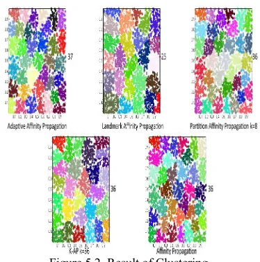
We also provide the sample result from each algorithm and original Affinity Propagation to be compared. We provide the result from test of 2000 data points in Fig.5.2. The interesting note here is how LAP as the fastest algorithm in test before has a less number of clusters than Affinity Propagationand thus, made it has a very different result of clustering. Other than LAP, all algorithms have almost same number of clusters as Affinity Propagation though K-AP is easily to acquire this number of clusters because of its usability.
Figure 5.2. Result of Clustering
6. CONCLUSION AND FUTURE WORKS
In this paper, we compare four Affinity Propagation expansion algorithms to clustering random two dimensional data points and finding best algorithm in speed. We also analyze it from theoretical perspective so the result from theoretical
analysis can support the result from running test. From theoretical analysis, we found that LAP (Landmark Affinity Propagation) has the most efficient computational cost than other Affinity Propagation expansion algorithms. The running test result shows LAP and PAP (Partition Affinity Propagation) with k=8 have the best time than other Affinity Propagation expansion algorithms. So, both theoretical analysis and running test showed that LAP has the best performance in the measurement of time.
Even though LAP has the best performance, LAP does not provide the best result as the result is quite biased compared to the original Affinity Propagation that already have low error. PAP with k=8 itself actually obtained quite a good result with a faster spent time than Affinity Propagation. Although LAP and PAP obtained a comparable result, it should be noted that LAP is better as computational cost so it has a better scaling in time than PAP.
The test is still need to improve, as the datasets is still a random data points. The suggestions from us for further research of this paper are as follows:
1. The test should use another type of data as Affinity Propagation can use many kind of similarity input, it can be a set of photo as example. If data points is still used on future research, the data should have several sets with different characteristics such as a dense or sparse sets.
2. The number of algorithms used in the test is still too few. Therefore, the test need to add other Affinity Propagation expansion algorithms.
3. The test in this paper is still lacking, therefore additional test is actually needed for further research. Several examples such as ARI (Adjusted Rand Index) and clustering error (CE).
ACKNOWLEDGMENT
The authors would like to thank the Gunadarma Foundations for financial supports.
REFERENCES
[image:8.612.102.289.442.631.2][2] Anon. (2010, Feb.) Data, data everywhere. http://www.economist.com/node/15557443. Accessed: 2016-03-24.
[3] S. M. Shamsuddin and S. Hasan, “Data science vs big data at utm big data centre,” in 2015 International Conference on Science in Information Technology (ICSITech), 2015. [4] J. Han, M. Kamber, and J. Pei, Data Mining:
Concepts and Techniques, 3rd ed. San Francisco, CA, USA: Morgan Kaufmann Publishers Inc., 2011.
[5] B. J. Frey and D. Dueck, “Clustering by passing messages between data points,” Science, pp. 972–976, 2007.
[6] J. Macqueen, “Some methods for classification and analysis of multivariate observations,” in In 5-th Berkeley Symposium on Mathematical Statistics and Probability, 1967, pp. 281–297. [7] Y. Fujiwara, G. Irie, and T. Kitahara, “Fast
algorithm for affinity propagation,” in
Proceedings of the Twenty-Second
International Joint Conference on Artificial Intelligence - Volume Volume Three, ser. IJCAI’11. AAAI Press, 2011, pp. 2238–2243. [Online]. Available: http://dx.doi.org/10.5591/ 978-1-57735-516-8/IJCAI11-373
[8] D. Xia, F. Wu, X. Zhang, and Y. Zhuang, “Local and global approaches of affinity propagation clustering for large scale data,” CoRR, vol. abs/0910.1650, 2009. [Online]. Available: http://arxiv.org/abs/0910.1650 [9] K. Wang, J. Zhang, D. Li, X. Zhang, and T.
Guo, “Adaptive affinity propagation clustering,” CoRR, vol. abs/0805.1096, 2008. [Online]. Available: http://arxiv.org/abs/0805. 1096
[10]R. Refianti, A. Mutiara, and A. Syamsudduha, “Performance evaluation of affinity propagation approaches on data clustering,” International Journal of Advanced Computer Science and Applications(IJACSA), vol. 7, no. 3, 2016.
[11]K. Zhang and X. Gu, “An affinity propagation clustering algorithm for mixed numeric and categorical datasets,” Mathematical Problems in Engineering, September 2014.
[12]Y. He, Q. Chen, X. Wang, R. Xu, X. Bai, and X. Meng, “An adaptive affinity propagation document clustering,” in Informatics and Systems (INFOS), 2010 The 7th International Conference on, March 2010, pp. 1–7.
[13]M. Rueda, M. A. Rodriguez, and B. A. Hawkins, “Identifying global zoogeographical regions: Lessons from wallace,” Journal of
Biogeography, vol. 40, no. 12, pp. 2215–2225, Dec. 2013.
[14]V. de Silva and J. B. Tenenbaum, “Sparse multidimensional scaling using landmark points,” Technical Report, 2004.
[15]X. Zhang, W. Wang, K. Nreg, and M. Sebag, “K-ap: Generating specified k clusters by efficient affinity propagation.” in ICDM, G. I. [16]Webb, B. L. 0001, C. Zhang, D. Gunopulos,
and X. Wu, Eds. IEEE Computer Society, 2010, pp. 1187–1192. [Online]. Available: http://dblp.uni-trier.de/db/conf/icdm/icdm2010. html#ZhangWNS10
[17]Y. Weiss, C. Yanover, and T. Meltzer., “Linear programming relaxations and belief propagation - an empirical study,” in Journal of Machine Learning Research, vol. 7, 2006, pp. 1887–1907.
[18]P. Galdi, F. Napolitano, and R. Tagilaferri, “A comparison between affinity propagation and assessment based methods in finding the best number of clusters,” in CIBB, Jun. 2014. [19]P. Galdi, F. Napolitano, and R. Tagliaferri,
Computational Intelligence Methods for Bioinformatics and Biostatistics: 11th International Meeting, CIBB 2014, Cambridge, UK, June 26-28, 2014, Revised Selected Papers. Cham: Springer International Publishing, 2015, ch. Consensus Clustering in Gene Expression, pp. 57–67. [Online]. Available: http://dx.doi.org/10.1007/978-3-319-24462-4_5
[20]L. Liu, X. Chan, D. Luo, and M. Liu, “Hsc: A spectral clustering algorithm combined with hierarchical method,” Neural Network World, vol. 23, no. 6, pp. 499–521, Jan. 2013.
[21] A. B. Mutiara and R. Waryati, “Implementa-tion and comparison of affinity propaga“Implementa-tion algorithm and k-means clustering data on student gpa and time based road to campus,” in E-Journal Teknologi Industri, 2012.
[22]M. J. Brusco and H.-F. Köhn, “Comment on "clustering by passing messages between data points",” Science, vol. 319, no. 5864, pp. 726– 726, 2008. [Online]. Available: http://science. sciencemag.org/content/319/5864/726.