CLASSIFICATIONS, ASSESSMENTS AND CHARACTERISTICS AS FACTORS TOWARDS ANALYZING ORGANIZATIONAL KNOWLEDGE

6608

LOCATION-AIDED LEVEL BASED DISJOINT MULTIPATH

ROUTING (LLDMR) ALGORITHM

1_{V.MUTHUPRIYA,} 2_S.REVATHI

1_{A.P (Sel.Gr), B.S.Abdur Rahman Crescent University, Department of CSE, India}

2 _{Associate Professor. B.S.Abdur Rahman Crescent University, Department of CSE, India}

E-mail: 1_{[email protected],} 2_{[email protected]}

ABSTRACT

The routing in a dense causes more routing overhead and end-to-end delay because of the broadcast storm problem and frequent link failure in the network. In mobile ad hoc networks, the broadcast of the Route Request (RREQ) packet among the nodes increases along with the increase in network size, which results in routing overhead. Similarly, in these networks, the rate of link failure increases with node speed and so the single path routing protocols reinitiate the route discovery phase to find a new path whenever there is a link breakage, which finally results in more end to end delay in the network. Though several reactive multipath routing protocols were been introduced to overcome this problem, it uses more RREQ broadcasting to identify multiple paths. Recently more location based routing schemes have been proposed in order to minimize these broadcast problem, but they are not scalable for large ad hoc networks. In this paper, Location-aided Level based Disjoint Multipath Routing (LLDMR) algorithm is proposed, which finds multiple node-disjoint paths between source and destination with minimum flooding of control messages. In the proposed algorithm, the RREQ broadcast occurs only within inter-link nodes to minimize control packet overhead. Also, the algorithm predicts the link failure by comparing the node's threshold value with link’s threshold value and accordingly it switches to alternate path even before the link failure occurs. The performance of LLDMR is analyzed using NS2 simulator by varying its network size and speed. The simulation results are compared with existing non-location based multipath routing protocol AOMDV and location based routing protocol, location aided route discovery mechanism based on two-hop neighbor information(TN-CMAD and TN-CRDN).. Also the simulation results show that the proposed system has a higher packet delivery ratio, a minimum of control packet overhead and a reduced end to end delay than the existing protocols, AOMDV, TN-CMAD and TN-CRDN.

Keywords: Location-Aided Routing (LAR), Location-Aided Level Based Disjoint Multipath Routing (LLDMR), Node-Disjoint Paths, Inter-Link Node, Node’s And Level’s Threshold Value.

1. INTRODUCTION

The Mobile Ad-hoc Networks are dynamic

infrastructure-less wireless networks. Each node of its network not only acts as a sender or receiver also acts a router, bridge, and gateway between different homogeneous or heterogeneous network. Since the transmission of data takes place in open unguided media they have several issues during packet transmission.

The conventional routing algorithms like Distance vector routing and link state routing are not appropriate for Ad hoc networks as these networks are dynamic in nature. So many routing algorithms based on proactive and reactive methods are developed for Ad hoc networks [1,2]. These existing methods have its own pros and cons. The flooding in reactive protocol and topology maintenance in proactive protocols increases the consumption of bandwidth to a considerable amount. The ad hoc

nature of the network sometimes leads to link failure, if there is only one path between source and destination then the route discovery process is again started. This results in a more end-to-end delay in the single path routing algorithms like Ad hoc On-Demand Distance Vector (AODV) routing [3] and Dynamic source routing(DSR) [6] in ad hoc wireless networks. So many research works were carried out to develop multipath routing algorithms like AOMDV [4,5], SMR[10], AODV-BR[9] , where on any link failure the communication take place through an alternate path. The multipath routing algorithms [8] involving RREQ flooding for path discovery has a major drawback of broadcast storm problem [7].

As said earlier in recent years many geographic or location based protocols like Location-Aided Routing(LAR)[13], Zone Based

6609 Protocol(ZHLS)[14] using Global positioning System (GPS) [15] has laid its landmark in finding paths for data transmission in Mobile Ad hoc networks. Nowadays most of the mobile devices are enabled with GPS and so usage of GPS has become quite common in minimum budget. Several

location-based mechanisms[11] were been

developed for detecting better positional accuracy of the target with minimum position error. In this paper, Location-aided Level based Disjoint Multipath Routing algorithm (LLDMR) is proposed where it finds the possible disjoint paths between source and destination using routing table information of the participating nodes.

The main advantage of the proposed algorithm is it finds disjoint multiple paths between the source and destination on-demand with minimum routing overhead and end-to-end delay. Since it finds disjoint multipath, the link failure on one route doesn’t affect the other and also the link failure is predicted even before it occurs and this notification is sent to the source node so that alternate path for packet transmission is easily chosen without any delay. The frequency of route updates is less when compared to other routing protocols due to the availability of disjoint paths and so decreases end to end delay in the network. The security issue is also another major reason for packet loss and end to end delay in mobile ad hoc network. The link failure due to routing attacks [12] is not considered in LLDMR and so attacker nodes are not considered in the simulation. The simulation results show the performance of LLDMR by varying its number of nodes and speed.

2. OVERVIEW OF LOCATION (GPS) AIDED

ROUTING PROTOCOLS

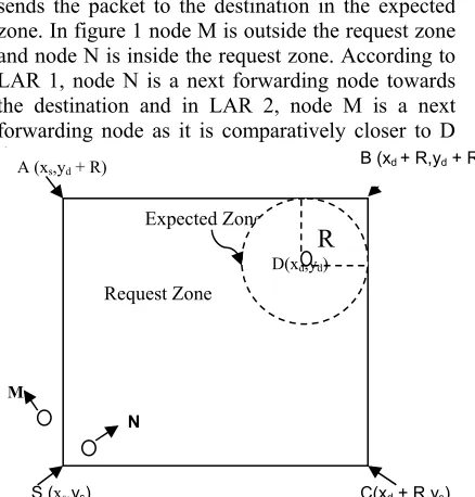
Location-Aided Routing (LAR) [13] is the location based routing algorithm which finds its routing path similar to DSR protocol. It reduces control message overhead in DSR[ 4] by searching the route only in the limited portion of the whole network. It introduces two algorithms LAR 1 and LAR 2 for efficient utilization of resources. In both the algorithms the destination location information is assumed and velocity of the destination node (D) is calculated. The initial location of node-D is D(xd,yd) at t0 and R is the distance traveled by the

node-D at t1 in either X or Y direction. Using this

information, the region of movement of the destination node in X direction is xd + R at t1and in

Y direction is yd + R at t1. So with R as radius and

D(xd,yd) as a mid-point, a circular region is drawn

and this region is the expected zone. By joining the

vertices S (xs,ys), A (xs,yd + R), B (xd + R,yd + R),

C(xd + R,ys), the planar region is found which

includes the expected zone in it. The region excluding the expected zone in the planar region is called request zone. The expected zone is the target zone for both LAR 1 and 2 and so the nodes in the request zone is alone used for flooding the RREQ towards expected zone. In LAR 2, the nodes which are a minimum distance from destination location are considered for flooding and using these nodes, it sends the packet to the destination in the expected zone. In figure 1 node M is outside the request zone and node N is inside the request zone. According to LAR 1, node N is a next forwarding node towards the destination and in LAR 2, node M is a next forwarding node as it is comparatively closer to D than N.

Figure 1. LAR routing scheme

GeoAODV [16,17], a variation of LAR, where it assumes the nodes know only their location information and they are unaware of the destination's location or traveling speed. In this cone shaped request zone is defined between the source and destination. The source node acts as an edge in the cone shaped request zone and the width of the cone is defined by flooding angle. A line evenly divides the flooding angle such that it connects source A and destination D. The node N in the request zone can rebroadcast the RREQ only if it forms an angle α between N, A and D less than half of flooding angle otherwise discarded. The two variations of GeoAODV are GeoAODV rotates and GeoAODV static protocol. The request zone is same in later whereas in the former it varies dynamically depending on the availability of intermediate node towards the destination. The cone edge is always the source node in Geostatic and Georotate the cone is formed by the intermediate node by having itself as a cone edge.

Request Zone

R

D(xd,yd)

A (xs,yd + R) B (xd + R,yd + R)

C(xd + R,ys) S (xs,ys)

N

6610 A Distance Routing Effect Algorithm for Mobility (DREAM) [18], is proactive GPS-aided routing protocol. Each node maintains a routing table which contains location information of all other nodes in the network. The source node finds the direction of the destination using destination node's location information and transmits the packet to its one-hop neighbors in that direction. These neighbor nodes repeat the same process till the packet reaches the destination. Since there is no route discovery phase, a considerable amount of delay when compared to reactive protocols are reduced. The location information of the nodes is updated in the network depending on the distance effect and mobility rate of the communicating nodes. It is bandwidth and energy efficient when compared to other proactive and reactive protocols.

Greedy Perimeter Stateless Routing (GPSR) [19,20], is a scalable proactive routing protocol. It uses the location information of the intermediate and the destination node to transmit the packet. It employs two methods for packet forwarding, namely greedy routing [15] and perimeter or face routing [16]. In greedy forwarding method, the node which is nearer to the destination is chosen to be the next packet forwarding node. In some cases, this may raise to a void situation where

the node becomes a local maximum in its geographic proximity where it cannot find any other neighbor node other than itself as a closer node to the destination. If such situation arises the forwarding node is chosen using perimeter forwarding method.

A Hierarchical Geographical Routing with Alternate Paths Using Autonomous Clustering for Mobile Ad Hoc Networks (Hi-GRAP) [21] forms different clusters among the set of nodes in the network. Each cluster will have a cluster head, where the Node ID of the cluster head is the cluster ID of the cluster member nodes. In most of the Location-aided routing schemes, it is assumed that the source node knows the location of the destination before route discovery phase. In practice, it is very difficult because there is a chance of a destination node move from its assumed position. So in Hi.GRAP routing scheme, the source node finds the location of the destination node by flooding Location REQuest (LREQ) on the network and getting Location REPly from the destination node (LREP). The major issues in this scheme are, the cluster-head and cluster formation involve some extra control overhead due to an exchange of control packets, MEmber Packet (MEP) and Member Ack Packet (MAP). Also, when the cluster member or head moves out of its cluster area, the new cluster

head and members need to be formed. This again increases the delay in the network. Since the route request and reply to the cluster members are always through cluster head, maintaining the cluster size also involves some time-consuming process.

A Beacon-Less Geographic Multipath Routing Protocol for Ad Hoc Networks (BGM) [22] is a Beacon-less geographic node disjoint multipath routing strategy. It uses location information of the neighbors and four-way handshake mechanism to identify its forwarding neighbors in different zones. It divides the whole network into different disjoint zones using elliptic curves and finds disjoint paths through each zone. The number of disjoint paths depends on a number of disjoint zones formed. Node-disjoint paths are more reliable when compared to link disjoint paths as node disjoint links are less likely to fail. In BGM the performance is analyzed for both with a beacon (BGM-BN) and without beacon (BGM-BL).

In the simulation result, BGM-BL shows the maximum packet delivery ratio and minimum control overhead and more end-to-end delay compared to the BGM-BN. Since BGM-BL avoids beacons for finding the next forwarding hop, the control overhead is comparatively minimized. The end-to-end is comparatively more in BGM-BL because BGM-BL exhibits a four-way handshaking process to find the forwarding region in beacon less transmission. This increases the time for selecting the next hop in BGM-BL, whereas BGM-BN can easily find the next hop for transmission without much delay using the neighbor table. In BGM if the assigned zone does not have any forwarding node, the data packet chooses forwarding node from the adjacent zone. This switching from interior region forwarding mode to boundary region forwarding mode is also one of the reasons for the increase in end-to-end delay in BGM. Moreover, it also increases the number of joint nodes (common nodes) in the multiple paths formed.

6611 davg(vx) is the average distance to destination(D)

from two-hop neighbors of the sender node.TN-CRDN uses one hop information of the sender node and selects the next forwarder node which has

maximum Pr(vx) to find the forwarder node, where

Pr(vx), the probability of a number of neighbors of

one-hop neighbor nodes. The main issues in this mechanism are,

 The average distance information alone is not enough to find the forwarder node in TN- CMAD.

 The discovery of two hop information using

two hello messages will increase the routing overhead.

 It raises the complexity of the network during the update of the two hop information at the time link failure.

 Since both the algorithm finds the only single route, the route discovery phase is reinitiated when there is a failure in discovered path. In general, the most of the location-based routing protocols uses the greedy algorithm to find the next forwarder node but it may sometimes lead to the

void situation as mentioned in GPSR [19]. The link

failure occurs frequently due to increase in node velocity in Mobile Ad hoc network. In single path algorithms when a link failure occurs at the time of packet transmission, there is a possibility of many packets being lost till the discovery of new route. So the packet delivery ratio decreases and reinitiating of route discovery phase increases the end-to-end delay. Even though some multipath location-based routing protocol exists, in these protocols finding multipath involves more control packet exchange which results in more routing overhead as the network size increases.

In order to overcome most of these issues, the Location Aided Level Based Disjoint Multipath Routing (LLDMR) algorithm is proposed in this paper. The proposed algorithm uses minimum control packet broadcasting and finds multiple disjoint paths. The performance of LLDMR is analyzed using NS2 simulator and compared with existing LAR routing algorithm Location-aided route discovery mechanism based on two-hop information [23]. The analysis shows LLDMR exhibit less routing overhead, maximum packet delivery ratio and minimum end-to-end delay.

3. LOCATION AIDED LEVEL BASED

DISJOINT MULTIPATH ROUTING

(LLDMR) ALGORITHM

The LLDMR algorithm discovers disjoint multipath between source and destination only using

information in a neighbor table and routing table. It employs GPS to find the location information of each node and uses only the intermediate nodes in request zone for finding the route. In general, the two types of multipath routing schemes are link and node disjoint multipath routing.

 Link-Disjoint Multipath: In the figure 2, there is no

common link, but may have a common node (C) in the routes found between the source (S) and destination (D).

Figure 2: Link-Disjoint Multipath

 Node Disjoint multipath: In the figure 3, there are

no common nodes and common links in the routes found between the source (S) and destination (D). All node disjoint multipath routing is link-disjoint but not vice versa.

Figure 3: Node-Disjoint Multipath

The proposed algorithm LLDMR finds node disjoint multipath routing and so there is no common link or node in the multiple paths founded. Since alternate disjoint paths are available, the link or node failure will not cause much end to end delay and packet loss during packet transmission in the network.

3.1 Network Model

The Mobile Ad hoc network is a undirected wireless network G = (V, E), where V is a set of wireless nodes and E is a set of Undirected links connecting these nodes. Each node in the network is assigned a unique identifier (id) and all the nodes are assumed to have same transmission range R. It is a GPS-enabled network model and so each node is aware of its location information i.e x and y coordinates in its two-dimensional axis. The notation P(x,y) represents location information of node P. The initial flooding is done to find the destination location and velocity. Based on the velocity of the destination the expected zone of it is found. Like

S C D

6612 LAR, the expected zone is the anticipated region, where the destination node can move in any of the direction within this region/zone during the period of data transmission. These expected zone nodes are also involved for RREQ broadcasting so that the route to the destination node is always maintained for the total period of data transmission.

3.2 Description OF LLDMR Algorithm

Initially, when the source node S wants to transmit a packet to the destination D, the source node floods Location Request (LREQ), which contains the source.id, destination.id and LREQ.seqno to the whole network and finds the location of the destination through Location Reply (LREP) message. LREQ.seqno is used to identify the LREQ sequence so that broadcasting nodes discards duplicate LREQ. The nodes also identify its neighbors and destination location information using the same LREQ. After finding the expected and request zone similar to LAR [9] protocol, the statuses of all the nodes in these zones are set as unvisited (0). Hereafter we use the term intermediate nodes for expected and request zone nodes. Now the every node in the identified zone knows source.id, destination.id, source(x,y) and destination(x,y), The proposed algorithm finds possible node-disjoint paths between source and destination with minimum routing overhead. The two main phases of the algorithm are

 Route Discovery

 Route Maintenance

During route discovery phasethe disjoint routes are established between source and destination and the route maintenance is enabled whenever there is a link failure prediction in the network.

Each node maintains one list and two tables, i.e. one neighbor list and two tables namely information database and routing table. The neighbor list of each node contains the information of its one-hop neighbors on receiving LREP message from them. If the destination moves away from its expected zone position, the LREP is activated, so that the intermediate nodes and source node can update the new destination(x,y). The contents of information database and routing table are explained in the section (3.2.1).

3.2.1 Route discovery phase

This phase constitutes two main processes: Level identification process and Route finding process. In the Level identification process, the algorithm divides the intermediate nodes into different levels based on the distance or transmission range with

respect to the destination node. This is done in order to avoid control packet overhead in the intermediate nodes and also avoids the formation of a loop while finding a path.

 i.) Level identification algorithm

After finding the intermediate nodes, the different levels between the source and destination node is founded. This step is initiated by the destination node towards source node. The destination node is an only Level-0 node and it finds all its one-hop neighbors in the direction of the source and sets all these nodes as Level-1 nodes. Since all intermediate node knows the destination(x,y), they can find their Levels by finding its distance from the destination(x,y). The level varies from 1 to N, depending on the distance between the source and destination.

If R is the transmission range in meters (ms) and if the distance of the node from destination is X (ms) then,

 Nodes are at Level-1, if X <= R from destination node

 Nodes are at Level-2, if X > R and if X < = 2R from destination node.

 Nodes are at Level-3, if X > 2R and if X <= 3R from destination node.

 The Nodes at Level-N, if X > (n-1)R and if X <= nR

 In this process, immediately after identifying Level

of the intermediate nodes, status of non-visited (0) nodes are updated to visited (1).This is done in order to avoid finding levels for already visited nodes and also it eliminates the formation of the loop in the routing path.

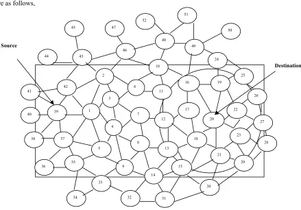
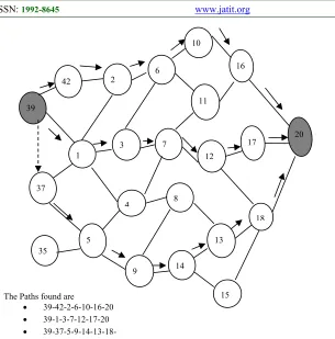
Consider the figure 4, where it is a wireless network and the link between the nodes represents that they are at one hop distance between them. In this network, the source node(39) wants to send a packet to the destination node(20). Like LAR-1 protocol the expected and request zones are identified. The circular region in the Figure. 4 is the expected zone, where the destination node(20) is likely to move in any direction within the zone during the period of full packet transmission. Depending on this expected zone, the request zone area i.e. the rectangular area is identified for RREQ broadcasting. The expected and request zone nodes together form intermediate nodes, where these nodes alone are involved in finding the route between source and destination.

6613 level. As a result of this process, there are seven levels in the network and the nodes under each level are as follows,

Figure 4: Link Representation of sample wireless Network

Level – 0 node: 20(destination node) Level – 1 nodes: 16, 17, 18

Level – 2 nodes: 10, 11, 12, 13, 15 Level – 3 nodes: 6, 7, 8, 14 Level – 4 nodes: 2, 3, 4, 9 Level – 5 nodes: 1, 5, 42

Level – 6 nodes: 35,37, 39 (source node)

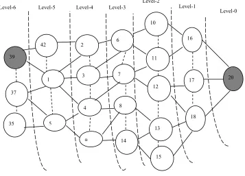
The figure 5 show the different levels of the intermediate nodes and also shows the inter-link and intra-link representation of the intermediate nodes and the table 1 shows the contents of intermediate nodes.

Table 1: Information Database

Parameter Value

Node. Level Level of the node

Status (0/1) Visited/ Unvisited node

Node(x,y) Node position

S.id Source id

S(x,y) Source position

D.id Destination id

D(x,y) Destination position

Inter link

nodes Neighbor node ids whose level no = Node. Level - 1 Intra-link

nodes

Neighbor nodes ids with level no – Node.Level

27 24

25

26

29

28 42

39

37

35 41

40

38

36

44 43

47

48

46

33

32 45

31

30 51

49

50

34

52

1 3

4

5

6 2

7

8

21 12

9

13

14 10

19

11

16

23

17 22

18

15

20

6614 ii.) Route finding algorithm

At this point, Inter link and Intra-link nodes are defined. Inter link: is the link or path formed between the nodes of level-n and level-(n-1). For ex: In Figure.5, the inter-link nodes of node-39 at level-6 are node-42 and node-1 at level-5.

Intra-link is the link or path formed between nodes of the same level... For ex: In Figure.5, at Level-1, the intra-link node of node-16 is a node-17 and intra-link nodes of node-17 are node-18 and node-16.

RREQ packet: It is the Route Request packet initiated by the source node and broadcasted towards the destination node. The RREQ packet contains,

 S.id: Source identification number

 D.id: Destination identification number

 RREQ.S.No: Route Request sequence number

Figure 5: Inter-Link And Intra-Link Representation Of Intermediate Nodes

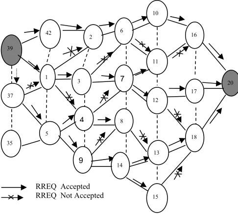
The figure 6 shows the route request broadcast for the network in Figure 5.The source node can broadcast to both inter and intra-link nodes. The intermediate nodes can flood only to its inter link nodes of the previous level and if there is no inter link node, it can flood to its intra-link nodes. For

ex, in the Figure 6 , if the intermediate node(42) does not have inter link node(2), it will flood the RREQ packet to the node(1). But node(1) will accept this RREQ only if it had not accepted the same RREQ packet earlier otherwise it discards this RREQ.

42

35 37 39

20 16

17

18 10

11

12

13

15 6

7

14 2

3

4

5 1

9

8

Level-0 Level-1

Level-2 Level-3

Level-4 Level-5

Level-6

6615 RREP packet: If the node accepts the RREQ packet, it sends the RREP to the sender node. Then the link between them is notified in sender routing table.

For ex: The RREQ from node(10) is accepted by node(16) and this is notified in the node(10) routing table in table 2.

Algorithms to discover Node-disjoint paths between Source and Destination:

Step 1: After identifying the intermediate nodes and their levels, the source node broadcasts the RREQ packet to its inter link and intra-link nodes.

Step 2: On receiving the RREQ packet, the intermediate node checks whether the route request is already accepted. If the RREQ is not

Figure 6: Route Request Broadcast

accepted previously, the intermediate checks whether it is the destination node or it has any route to the destination node in its routing table.

 If the intermediate node is the destination node, it sends RREP packet to the sender for notification of link in the routing table.

 Else If it has the route to the destination node in the routing table, it passes the information to the sender.

 Else it broadcasts the RREQ to its inter-link nodes. Step 3: Destination node alone accepts the duplicate RREQs from different inter-link nodes.

The node at each level maintains a routing table, where it stores path information to the destination through Interlink nodes of the previous level. Table 2 shows the details of the routing table of each level node in the network. In this source node(39) routing table shows two paths through inter- link and one path through intra-link node-37, to the destination node(20).

The three paths are 39-42-2-6-10-16-20, 39-1-3-7-12-17-20 and 39-37-5-9-14-13-18-20 respectively. These paths are node disjoint paths where no nodes or links are common in any of this path.

The figure 7 shows possible node disjoint paths in the network after implementing LLDMR algorithm. The RREQ is now flooded from source to its neighbors in the direction of destination from one level to another. Unlike AOMDV, duplicate RREQ are discarded by the nodes in order to minimize the control packet overhead during route discovery phase. Only the source node can send the RREQ to all the inter-link and intra-link nodes. The intermediate nodes send the RREQ only to Interlink nodes whose level is one lesser than it and only if there are no interlink nodes it broadcasts the RREQ to its intra-link node. This also minimizes the control packet overhead.

RREQ Accepted RREQ Not Accepted

35 37

42

39

2

3

4

5 1

9

6

7

14 8

20 16

17

18 10

11

12

13

6616

Figure 7: Node-disjoint Multipath

Table 2: Routing Table at each node’s-level

Node Interlink _{nodes notification} RREP Interlink _Path

Level-1 nodes

16 20 16 – 20 16 – 20

17 20 17 – 20 17 – 20

18 20 18 - 20 18 - 20

Level-2 nodes

10 16 10 – 16 10 – 16 - 20

11 16 RREQ( N.A) No path

12 17 12 – 17 12 – 17 - 20

18 RREQ(N.A) No path

13 18 13 – 18 13 – 18 - 20

15 18 RREQ(N.A) No path

Level -3 nodes

6 10 6-10 6-10-16-20

11 RREQ( N.A) No path

7 11 7-11 No path

12 7-12 7-12-17-20

8 13 RREQ( N.A) No path

14 13 14-13 14-13-18-20

15 14-15 No path

Level – 4 nodes

2 6 2-6 2-6-10-16-20

3 6 RREQ( N.A) No path

7 3-7 3-7-12-17-20

4 7 RREQ( N.A) No path

8 4-8 No path

9 8 RREQ( N.A) No path

14 9-14 9-14-13-18-20

Level-5 nodes

42 2 42-2 42-2-6-10-16-20

1 2 RREQ( N.A) No path

3 1-3 1-3-7-12-17-20

4 RREQ( N.A) No path

5 4 5-4 No path

9 5-9 5-9-14-13-18-20

Level-6 nodes

39 42 39-42 39-42-2-6-10-16-₂₀

1 39-1 39-1-3-7-12-17-₂₀

37 1 RREQ( N.A) No path

5 37-5 * 39 -37-5-9-14-_13-18-20

35 5 RREQ not sent No path

REQ(N.A) – Route Request is Not Accepted by Interlink node.

* path through the intra-link node.

3.2.2 Route Maintenance

Due to dynamic nature of mobile ad hoc networks, the nodes are free to leave and join the network. This is the major cause of link failure in mobile ad hoc network. Unlike other reactive multipath algorithms, the source node of LLDMR chooses the alternate path for packet transmission even before link failure is to happen. Based on the node's threshold value, each node predicts itself whether it enters or not into the critical section. 42

39

The Paths found are

 39-42-2-6-10-16-20

 39-1-3-7-12-17-20



39-37-5-9-14-13-18-37

35

20 16

17

18 10

11

12

13

15 6

7

14 2

3

4

5 1

9

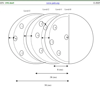
6617 Here the critical section is defined as the possibility of the node to move out from its current level to previous or next level. Figure 8 shows the different levels between the source node(S) and the destination node(D). In this figure the region after the vertical line is not considered for broadcasting according to LLDMR. The boundary of the critical section is marked with the dotted curve and the critical section is shown by the dotted arrow.

The minimum and minimum threshold value of each level is defined in equation 1 and equation 2 as follows,

TH-MIN (Leveln) =

. , ,

, , , (1)

TH-MAX(Leveln) =

. , ,

, , , (2)

Table 3: List of Abbreviations

Acronym Expansion

TH-MIN (Leveln) the maximum threshold of

Level- n, where n varies from 1 to N.

TH-MAX (Leveln) the minimum threshold of

Level-n,

where n varies from 1 to N

S(x,y) location of the source node

D(x,y) location of the destination node

Max.Dist

(Level-n, D(x,y)) the maximum distance between Level-n and D(x,y)

Min.Dist

(Level-n, D(x,y)) the minimum distance between Level-n and D(x,y)

Dist(S(x,y),D(x,y)) distance between source and the destination node

Nodemn m is the Node-id and n is

the level of the Nodem, m

varies from 1 to M

The intermediate nodes distance from the destination node with respect to its level always lies between the maximum and minimum distance of its level-m from the destination. If the Nodemn does not

satisfy this, it is likely to be in critical section i.e, moved out of its level to adjacent level.

According to LLDMR this situation is predicted earlier by finding node’s threshold value. The node’s threshold value is defined in equation 3 as follows,

TH (Nodemn) = _{, ,}, , _, , (3)

Also, constant value C is defined as a change of threshold value of the node for every second. C =

, , , (4)

Where M is the maximum distance a node can travel per second.

The two cases for prediction of link failure are,

Case 1: if the TH (Nodemn) > (TH-MAX (Leveln) -

C), then the Nodemn is nearing Level-n+1).

Case 2: if the TH (Nodemn) < (TH-MIN (Leveln)

+ C), then the Nodemn is nearing Level-(n-1).

 Example Scenario:

Consider the figure 9 and figure 10, let us assume

 Dist(S(x,y), D(x,y)) = 700 m

 R = 250 m

 M = 40 m

 C = 0.05

Then the Min.Dist(Level-n, D(x,y)),

Max.Dist(Level-n,D(x,y)), TH-MIN (Leveln) and

TH-MAX (Leveln) for each level using equation 1

and equation 2 are given in table 4.

Case 1:

Assume that, at the time t0 the node-7 which is in

level-1 is 200(ms) from the destination D and it moves at the speed of 40(m/s) away from D. So after 1(s) at the time t1 the distance of node-7 is

240(ms) from D. The threshold value of node-7 at time t0 and t1 using equation 3are 0.29 and 0.34,

where 0.34 > (0.36 – 0.05), which means node-7 is in critical section and it is nearing level-2.This is shown in figure 9, where the node-7 lies in the critical section at time t1.

Case 2:

Assume that, at the time t0 the node-3 which is in

level-2 is 300(ms) from the destination D and it moves at the speed of 40(m/s) towards D. So after 1(s) at the time t1 the distance of node-4 is 260(ms)

from D. The threshold value of node-3 at time t0

and t1 using equation 3are 0.43 and 0.37, where

0.37 < (0.36+ 0.05), which means node-3 is in critical section and it is nearing level-1.This is shown in figure 10, where the node-4 lies in the critical section at time t1.

6618 into the critical section and so gives notification to source node through its inter-link nodes. The source node on receiving this notification switches over to alternate route for packet transmission. Therefore in LLDMR, the source chooses the alternate path even before the link failure is to happen and so it avoids dropping of packets at the time of link failure. This enhances the reliable transmission in LLDMR and also it increases Packet Delivery Ratio.

Table 4: Minimum And Maximum Threshold Value At Each Level.

Figure 9: Node-7 from Level-1 is nearing Level-2

Level-n Min.Dist (Level-n, D(x,y))

Max.Dist (Level-n, D(x,y))

TH-MIN (Leveln) TH-MAX

(Leveln)

1 1 250 0.001 0.36

2 251 500 0.36 0.71

3 501 750 0.72 1.07

5

6

7 3

4 1

S D

8 2

Level-0 Level-1

Level-2 Level-3

R (ms)

3R (ms) 2R (ms)

6619

Figure 10: Node-3 from Level-2 is nearing Level-1

3.3 Result and Performance Analysis

3.3.1 Simulation Environment

The proposed algorithm LLDMR is simulated using NS2.35. The NS2 simulation parameters are given in table 5.

Table 5: NS2 Simulation parameters

Parameter Type Value

Simulator NS 2.35

Channel Type Wireless

Propagation model Two Ray Ground

Mobility Model Random way point

Network interface type(netif)

Phy/WirelessPhy

MAC type(mac) IEEE 802.11

Interface queue type (ifq) DropTail/PriQueue

Antenna model Omni Antenna

Max packet in ifq 50

Number of mobile nodes 30, 50 100,150

(node density)

Speed of the mobile nodes 0,5,10,15,20,25,30,35 ,40 m/s

X&Y dimension of topology

1000 x 1000 m2

Traffic Source CBR

CBR packet size 512 bytes

Transmission range 250 m

Pause Time 2 s

Simulation Time 900 

3.3.2 Performance Metrics

The performance of LLDMR was analysed for the following metrics using NS2.

 Average End to End delay: The average

end to end delay is normally defined as the average time taken for a packet to reach the destination node from the source node.

 Routing packet overhead: The routing

packet overhead in LLDMR is the control packet overhead due to route discovery 3

5

6

7 3

4 1

S D

8 2

Level-0 Level-1

Level-2 Level-3

R (ms)

6620 parameters like the broadcast of LREQ, LREP, RREQ and RREP control packets and periodic beacon messages between neighbour nodes.

 Number Of Hops: The average number of

hops is the average path length required for transmission of all the packets from source to destination.

 Packet Delivery Ratio: The Packet

Delivery Ratio(PDR) is defined as the ratio of a number of packets received at the destination node to the number of packets sent from the source node. 

3.3.3 Simulation results

 Average end to end delay:

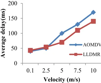
In any reactive routing protocol during packet transmission, as the velocity of the node increases the link failure also increases which finally ends up with more end to end delay.

Figure 11(a): Average End to End Vs. Velocity

Figure 11(b): Average End to End Vs. Velocity

Figure 12: Average End to End delay Vs. Number of nodes

The figure 11(a) shows at higher node density, the LLDMR has comparatively less end to end delay than AOMDV. In mobile ad hoc networks, the link failure rate increases with increase in node mobility and this finally results in more end to end delay in the network. Since LLDMR can predict the link failure in advance, the notification to source node and switching to alternate path happens simultaneously with ongoing packet transmission process. Unlike AOMDV, LLDMR need not wait till link failure time and choose the alternate path for packet transmission. So as shown in figure 11(a), LLDMR has comparatively lesser end to end delay than AOMDV. In figure 11(b) and Fig 12, the average end to end delay of LLDMR with respect to velocity and number of nodes are compared with existing technique TN-CMAD and TN-CRDN.

In the route discovery of the proposed algorithm, the end to end delay includes the node’s level identification period, broadcast time of RREQ and RREP packets. After finding the intermediate nodes between source and destination and knowing the destination’s position, these intermediate nodes can identify its level simultaneously using level identification algorithm.

So when the node density increases, the

level identification process is not going to affect much the end to end delay whereas the node movement causes some influences in network delay. As the distance between the source and the destination increases the number of levels also increases, this causes more inter-node broadcasting of RREQ and RREP. But still, the algorithm exhibits comparatively less end to end delay at higher node density and velocity than TN-CMAD and TN_CRDN. This is because intra-node broadcasting is totally avoided in LLDMR. Also, 0

50 100 150 200

0.1 2.5 5 7.5 10

Average

d

el

ay(ms)

Velocity (m/s)

AOMDV

LLDMR

0 0.2 0.4 0.6 0.8 1 1.2

0 5 10 15 20 25 30 35 40

Average

E

nd

to

E

nd

delay

(s)

Velocity (m/s) TN-CMAD TN-CRDN LLDMR

0 0.01 0.02 0.03 0.04 0.05

30 50 100 150

Average

E

nd t

o

End delay

(s

)

Number of nodes TN-CRDN

6621 LLDMR finds multiple disjoint paths, so the link failure during packet transmission uses alternate path for transmission instead finding a new route.

 Routing packet overhead:

Figure 13:. Number of Overhead Vs Number of Nodes

The figure 13 shows at sparse network the routing packet overhead is more in LLDMR than existing technique TN-CMAD and TN-CRDN, due to above-said route discovery parameters. But at the dense network, though these parameters exist, the routing packet overhead is comparatively lesser than existing technique.

This is because in existing technique TN-CMAD and TN-CRDN, apart from these route discovery parameters, each node will broadcast two times hello messages, first for getting one-hop information and second for getting two-hop information. Hence when the number of node increases, the number of hello messages broadcasted will also be double the number of nodes, which causes more routing packet overhead at higher node density. The main scope of LLDMR algorithm is to reduce the routing packet overhead at dense networks by using minimum flooding during route discovery phase. This is achieved in LLDMR by just having only inter-level broadcasting of RREQ and RREP packets and exchanging beacon messages only with one-hop neighbors.

 Number of hops:

In LLDMR, when the node density is less, finding the path directly with the inter-level nodes is difficult and so it may take the path through intra-

Figure 14: Number of Hops Vs Number of Nodes

level nodes. Thus in LLDMR, the path length increases as the node density decreases. This is shown in figure 14 where, when the number of the node is 30, the LLDMR has higher path length than TN-CMAD and TN-CRDN. But in LLDMR, when the number of nodes gradually increases, the number of hops eventually decreases. Finally, at high node density in Fig 14, the proposed algorithm comparatively requires a minimum number of hops for packet transmission than TN-CMAD and TN-CRDN.

 Packet delivery ratio:

The figure 15 shows the PDR is always high for LLDMR when compared to CMAD and TN-CRDN due to the availability of multiple disjoint paths.

Figure 15. Packet Delivery Ratio Vs. Velocity

According to the proposed algorithm, the nodes can predict their breakage from the current path 0

100000 200000 300000 400000 500000 600000 700000 800000 900000 1000000

30 50 100 150

Number

of overhead

(packets)

Number of nodes TN-CRDN TN-CMAD

LLDMR 0

10 20 30 40 50

30 50 100 150

Num

b

er

o

f hops (hops)

Number of nodes TN-CRDN TN-CMAD LLDMR

0 10 20 30 40 50 60 70 80 90 100

0 5 10 15 20 25 30 35 40

Packet

D

elivery

R

atio

(%

)

Velocity (m/s)

TN-CMAD

TN-CRDN

6622 using its minimum and the maximum threshold value. If it predicts that it is in a critical section, the notification is sent to the source node through the inter-link nodes. So source node immediately chooses an alternate path for packet transmission instead, thus it avoids a packet being dropped due to link failure.

In figure 16 the packet delivery ratio is always less in sparse networks than in dense networks in both existing and proposed algorithms. It is because sometimes sender node could not find a forwarding node immediately in the sparse network and so packets may be dropped before reaching the destination. The existing technique TN-CMAD and TN-CRDN computes the forwarding node based on the distance between the forwarding node and destination.

Since the nodes can move freely in the mobile ad hoc network, there is a chance for the

void [19] situation in the network. This rarely

happens in LLDMR due to the availability of alternate paths for packet transmission. When the node density increases the links between the nodes are very strong and so the packet delivery ratio increases.

Figure 16. Packet Delivery Ratio Vs. Number of Nodes

4. CONCLUSION

Location based routing algorithms have very much minimized the control packet overhead in reacting routing protocols. In this paper, location based routing algorithm LLDMR is proposed which finds node disjoint multiple path between the source and destination nodes with minimum flooding. The broadcasting of RREQ packets is limited only to

inter-link nodes and thus the control packet overhead is considerably reduced in LLDMR. The LLDMR algorithm shows relatively lesser end to end delay than existing non-location based multipath reactive routing protocol AOMDV and minimum control packet overhead than location based multipath routing protocol TN-CMAD and TN-CRDN. During link failure, the existing multipath routing algorithms chooses the alternate path only after the link failure happens in the network whereas the LLDMR chooses the alternate path even before the link failure happens by predicting it in advance. So it proves minimum end to end delay compared to existing multipath routing algorithms, AOMDV, CMAD and

TN-CRDN. Also LLDMR overcomes void [19]

situation, the most significant issue in greedy based routing algorithms. As for the future work it is planned to extend the LLDMR algorithm to overcome routing attacks and ensure secure packet transmission without any packet loss.

REFERENCES

[1] Saleh Ali K. Al-Omari, Putra Sumari, ” An overview of Mobile Ad Hoc Networks for the

existing protocols and applications,”

International Journal on applications of graph theory in wireless ad hoc networks and sensor networks (Graph-Hoc), Vol.2, No.1, March 2010.

[2] X.Hong, K. Xu, and M. Gerla, "Scalable Routing Protocols for Mobile Ad Hoc Networks," IEEE network, pp. 11-21, July/August 2002.

[3] Perkins C., Royer E. B., and Das S., "Ad hoc

On-Demand Distance Vector (AODV)

Routing - Internet Draft", IETF Network Working Group, RFC 3561, pp.1-38, 2003.

[4] M.K. Marina, S.R. Das, "On-demand

Multipath Distance Vector Routing in Ad Hoc Networks", Proceedings of the International Conference on Network Protocols, 2001. [5] M. K. Marina and S. R. Das, " Ad hoc On-

demand Multipath Distance Vector Routing ",

Technical Report Computer Science

Department, Stony Brook University, 2003. [6] Johnson, D., And Maltz, D. A.," Dynamic

source routing in ad hoc wireless networks", in

Mobile Computing, T.Imielnski and H. F.

Korth, Eds. Kluwer Academic Publishers, Dordrecht, the Netherlands, 1996, ch. 5, pp. 153-181.

97.5 98 98.5 99 99.5 100 100.5

30 50 100 150

Packet

D

elivery

R

atio

(%

)

6623 [7] S.-Y. Ni, Y.-C. Tseng, Y.-S. Chen, and J.-P.

Sheu, ”The Broadcast Storm Problem in a Mobile Ad hoc Network”, Int'l Conf on

Mobile Computing and Networking

(MobiCom'99), pp. 151-162, 1999.

[8]Tarique M, Tepe KE, Adibi S, Erfani S,

“Survey of multipath routing protocols for mobile ad hoc networks”, Journal of Network and Computer Applications 32(6):1125–1143, 2009.

[9]Lee SJ, Gerla M,"AODV-BR: backup routing in

ad hoc networks", In Wireless

Communications and Networking Conference, WCNC. 2000 IEEE, 2000 (vol. 3, pp 1311– 1316 vol.1313), 2000.

[10]Lee SJ, Gerla M(2001), "Split multipath routing with maximally disjoint paths in ad hoc networks", In Comminications. 2001. ICC 2001. IEEE International Conference, vol. 10, pp. 3201-3205,2001.

[11]E. Kuiper, S. Nadjm-Tehrani, " Geographical Routing With Location Service in

Intermittently Connected MANETs ", Vehicular Technology, IEEE Transactions on, vol.60, no.2, pp.592-604,2011

[12]V.Muthupriya And K. M. Mehata,

”Performance Analysis of AOMDV under the impact Of Rushing Attack”, International Journal Of Applied Engineering Research Issn 0973-4562 vol.10, no.11 (2015), pp. 29581-29594.

[13]Y. Ko and N. H. Vaidya, "Location-aid routing (LAR) in mobile ad hoc networks", Wireless Networks, vol.6, pp.307-321, 2000.

[14]M.Joa-Ng and L.T.Lu. " A Peer-to-Peer Zone-Based Two Level Link State Routing Protocol for Ad hoc Networks", IEEE Journal on Selected Areas in Communications, vol. 17, no. 5, pp. 1415-1425, 1999.

[15]Kaplan, E. D., Ed. Understanding GPS:

principles and applications. Artech House,

Boston, MA, 1996.

[16]Hnatyshin, and H. Asenov, "Design and Implementation of an OPNET model for simulating GeoAODV MANET routing protocol", Proc. of the OPNETWORK 2010 International Conference, Session: Wireless Ad Hoc and Wireless Personal Area Networks, Washington DC, 2010.

[17]H. Asenov, and V. Hnatyshin, "GPS-Enhanced AODV routing", in Proceedings of the 2009

International Conference on Wireless

Networks (ICWN'09), Las Vegas, Nevada, USA (July 13-16, 2009).

[18]S. Basagni, I. Chlamtac, V. R. Syrotiuk, and B. A. Woodward, "A Distance Routing Effect Algorithm for Mobility (DREAM)",

ACM/IEEE International Conference on Mobile Computing and Networking (MobiCom), Dallas, TX, pp. 76-84, 1998.

[19]B. Karp and H. T. Kung, "GPSR: greedy perimeter stateless routing for wireless networks”, in MobiCom’00, pp. 243–254, 2000.

[20]Y.J. Kim, R. Govindan, B. Karp, and S. Shenker, “Geographic routing made practical”, in Proceedings of 2nd Symposium on

Networked Systems Design and

Implementation. USENIX, 2005, pp. 217–230.

[21]Hiroshi Nakagawa, Satoshi Teshima,

Tomoyuki Ohta, Yoshiaki Kakuda, “A Hierarchical Geographical Routing with

Alternative Paths Using Autonomous

Clustering for Mobile Ad Hoc Networks”, IEICE Transactions on Communications 94-B(1):37-44, 2011.

[22]Ping Dong, Huanyan Qian, Xiaofei Wei,

Shaohua Lan & Cunlai Pu, "A Beacon-Less Geographic Multipath Routing Protocol for Ad Hoc Networks Mobile Networks and Applications”, 18(4), 2013.