AN EMPIRICAL EVALUATION FOR THE INTRUSION DETECTION FEATURES BASED ON MACHINE LEARNING AND FEATURE SELECTION METHODS

6116

EEG BASED USER IDENTIFICATION METHODS

USING TWO SEPARATE SETS OF FEATURES BASED ON

DCT AND WAVELET

1_{HEND A. HADI}* _, 2_{DR. LOAY E. GEORGE}

1,2_{College of Science, Computer Science Department, Baghdad University, Baghdad, Iraq}

Emails: 1_{[email protected] ,} 2 _{[email protected]}

ABSTRACT

Brain activities may represented by EEG signals, which are set of measures using electrodes along the scalp, they are more secret, sensitive, and hard to steal and reproduce. They hold great potential to provide robust and secure biometric system for user identification and verification. This paper aims to present a comparison between our previous proposed feature set that based on Partitioned Fourier spectra and some new features sets proposed in this work. They established as simple, fast, and promising set of features for EEG-based identification system. The first introduced feature set is based on the e

nergy distribution

Each proposed method was tested using the publicly available EEG CSU dataset which was collected from seven healthy volunteers and the publicly available EEG Motor Movement/Imagery dataset which is relatively large dataset was collected from 109 healthy subjects. The attained identification results are encouraging with best recognition rate is (100%) for all proposed methods and for both datasets. All tested feature sets were extracted under the condition, which was adopted in our previous work, that is "they should extracted from EEG data belong to single task & signal channel". All achieved results are considered competitive when compared with the results of other recently published works. The adopted condition reduced the computational complexity and thus reduced the required processing time. Also, the wavelets based methods hold computational complexity less than DFT and DCT with recognition rates are more competitive to them.

Keywords: Signal Processing, Wavelet Transforms, DCT, Energy Features, And Statistical Moments.

1.INTRODUCTION

Biometric traits of the human Electroenceph-alogram (EEG) have received great interest from some scientific researchers. The very beginning of the human EEG recordings was by Hans Berger in 1924, these signals are used to diagnose many diseases, especially those affecting the brain [1]. Recently EEG traits used for automatic identif-ication and verifidentif-ication of individuals; EEG traits show robustness against falsification and repli-cation more than traditional biological traits [2], [3].

Palaniappan (2016) Proposed to use EEG signals from 6 channels for each mental task to maximize inter-classes differences, the features were extracted from AR coefficients, channel spectral powers,

inter-hemispheric channel spectral power differ-ences, linear and the non-linear complexity of inter-hemispheric channel, the total features (108) after filtering the signals using Finite Impulse Response (FIR) high-pass filter to remove baseline noise, after that he used Principal Component Analysis (PCA) to reduce feature vector size, finally he classified five subjects from (CSU dataset) using LinearDiscriminant Classifier(LDC and achieved recognition rate up to (100%) with features combined from Rotation, Math., Letter, Baseline tasks [4].

6117 order to classify 7 subjects of CSU dataset; they used (LVQNN) and its extension LVQ2. The best recognition rate that they achieved is (96.05%) [5]. Daria La Rocca et al. (2014) introduced a novel approach which is based on the fusion of spectral coherence-based connectivity; they explored EC and EO resting conditions mental tasks and fused features from two channels for a single task. They used PSD and Spectral Coherence Connectivity for feature extraction, they classified (108) subjects from Motor Movement/Imagery dataset using a Mahalanobis distance-based classifier, the best attained result was (100%) [6].

Rodrigues et al. (2016) explored the minimizing of electrodes needed to identify users; they evaluated a binary version of the Flower Pollination algorithm to select best subset of electrodes that lead to best accuracy using Optimum-Path Forest classifier. They maintained recognition rate up to (87%) using half of electrodes number [3]. Kumari and Vaish (2015) explored the ability of motor movement and imagination cognitive tasks to identify subjects, they used different methods of Daubechies wavelet transform and different energy methods was applied for each sub-band to extract features, then they use Back Propagation ANN to classify 5 subjects from Motor Movement/ Imagery dataset. They achieved (TAR=95%) as a best result, and proved in their study that Motor Imagery cognitive tasks has better applicability than Motor Movement tasks [7]. In our proposed work the used Daubechies (db4) wavelet transform was considered with two types of statistical moments in which the statistical moments are applied on each sub-band, and the statistical distance measure was adopted for matching stage. This leads to less complexity and little computational time require-ment.

Yang et al. explored the sensitivity of EEG biometric recognition to the type of mental tasks which the tested subjects perform while their EEG signal is being recorded. Also they study the effect of using one task for training and another one for testing. They investigated the fusion of features from different tasks and electrodes for best recognition rate. The wavelet packet decomposition (WPD) was used for feature extraction; specifically they used (Daub4) packet decomposition, and then the standard deviation of each enhanced sub-band was calculated as feature element. Features from different tasks and electrodes (9 electrodes) were fused to generate the final features vector, then they fed to LDA classifier to classify (108) subjects from Motor Movement/Imagery dataset, the best achieved CRR was (99%) [8].

However, the previous researches on EEG-based recognition faced the problem of the used number of electrodes and mental tasks to discriminate subjects, more than one task and many electrodes lead to make the acquisition process more complex, also faced complications in feature extraction and in their fusion to make appropriate feature vector that is fed to the classifier.

In order to make the EEG-based biometric system applicable and usable, the number of electrodes andtasks requiredshouldbe reducedto minimize the complexity of EEG signal acquisition from the scalp of the user, as well as the complexity of the system and the processing time should be reduced by using feature extraction methods and classifiers with least computational complexity [2]. In this research paper the use of minimum number of tasks and channels (i.e., one channel per task) was adopted and investigated to achieve high recognition accuracy without the need to costly features fusion phase, and to keep the required computational complexity as low as possible. Two separate feature sets are proposed in this research, first set is based on the energy of sliced power spectra of DFT and DCT, while the second set of features based on the calculation of the statistical moments of wavelet sub bands; three types of wavelet transforms are proposed: Haar wavelet transform, Daubechies (db4), and bi-orthogonal (Tap9/7) each one of them has a relatively minor computational complexity. The discrimination strength of the introduced features was analyzed, combined using LDA, and the normalized Euclidean distance measure was used in matching stage.

2.MATERIALS AND METHODS

The proposed EEG-based identification system is based on the following main stages for identification purpose:

1. Mapping from time to frequency domain stage. 2. Feature extraction stage.

3. Feature analysis and selection stage. 4. Matching stage.

In mapping stage different transform methods were proposed in the literature; in this paper the input EEG signal is mapped into frequency domain to extract the main discriminating features.

6118 In matching stage some Euclidean distance measures are used to decide the closeness of samples and subjects identity.

2.1 Dataset

Two public datasets are used in this paper project:

2.2.1 EEG CSU dataset

This is a public dataset was collected by Keirn and Aunon [9]; and freely available at [10]. It is a small dataset which consists of the EEG recordings of seven healthy subjects. Each subject hadperformedsomementaltasks. These tasks are: Baseline task, Letter composing task, mathematics task, rotation task, counting task. Signals were recorded from the positions C3, C4, P3, P4, O1 and O2; see Figure 1. The taken EEG signals duration is 10 sec. with sampling rate (250 sample/sec) [2]. The tested tasks are:

 Baseline task: in this task each subject sat in relaxation state with eyes open or closed [9].  Mathematics task: the subjects were asked to do

some multiplication operations without doing physical activities or even saying anything [9].  Geometric rotation of a figure task: the subjects

imagined any three dimensional object, after that imagined the rotation of this figure around a particular axis [9].

 Letter composing task: in this task volunteers mentally composing letters without vocalizing.  Counting task: volunteers in this task asked to

count a series of numbers visually [9].

This dataset holds an error that occurred in one of subjects (i.e., 4th_{) in letter composing trails}

[5], [9].

2.2.1 Motor Movement/Imagery dataset

This is a large dataset consists of EEG recordings for 109 healthy persons; it was described in [11], and freely available on [12]. In this dataset the participantsranout14attemptsofthefollowing 6 tasks:

a. Baseline task with eyes open b. Baseline task with eyes closed c. Task1 (open and close left/ right fist).

d. Task2 (imagine the opening and closing of left/right fist).

e. Task3 (open and close both fists and both feet).

f. Task4 (imagine opening and closing both fists and both feet).

Each participant performed the first two tasks (baseline tasks) one time and performed the other tasks (Task1-Task4) three times (in same order). The signal data of all attempts are available in separated files with (EDF) file format. The

dataset contains the recordings of 64 channel based on 10-20 international system of electrode placement as shown in Figure 1 The recording duration is ranging from 1 minute to 2 minutes except for subject (106) who performed task3 for (36 sec. and 294 msec.) in attempt 5; the EGG recording was sampled at (160 Hz) [11] [13].

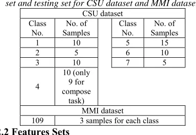
Table 1 shows the number of samples for each subject class in CSU dataset (CSU dataset) (Note: subject 4 has 9 samples for the letter-composing task because of the error that abovementioned), and the number of samples for each subject class in MMI dataset (Motor Movement/imagery dataset).

Figure 1: The (10-20) international system of electrode placement [3]

Table 1: Number of samples for each class for training set and testing set for CSU dataset and MMI dataset

CSU dataset Class

No.

No. of Samples

Class No.

No. of Samples

1 10 5 15

2 5 6 10

3 10 7 5

4

10 (only 9 for compose

task)

MMI dataset

109 3 samples for each class

2.2 Features Sets

In this stage, firstly a time-to-frequency domain mapping step is applied using some proposed transform methods. Then, the energy based features and/or the statistical moments features are used to generate feature vector. The considered transform domains are:

6119  Discrete Wavelet Transforms

 Haar Wavelet Transform (HWT)  Daubechies Wavelet Transform (db4)  Bi-orthogonal Wavelet Transform (Tap9/7)

2.2.1 Energyof Sliced Discrete CosineTransform (DCT) Spectra

Mapping a finite sequence of data points of EEG signal from a time-domain to a sum of cosine functions oscillating at different frequencies, it is a Fourier related but just using real numbers [14]. The DCT general mapping equation is given by:

DCT consists of (DC) and (AC) coefficients just like Fourier, (DC) is the first coefficient in index (0) which refers to the mean of signal; other components are the alternating components (AC). The high frequency components exist at the end of transform signal, while the low AC-frequencies are concentrated at the beginning [15].

After DCT step, then the obtained (AC) coefficients are divided into a number of blocks (or bands) and the energy of each block is calculated by taking the average of each block, the energy average of each block is given by the Eq. (2) [16]:

Where the energy of jth _block; N _{is the}

number of energy blocks,s is the index of the first coefficient belongs to jth _{block; L is number of}

coefficients belong to this block. Each block average, en(j), represents one feature.

2.2.2 Statistical Moments of Discrete Wavelet Transforms

DWT decomposes the signal into frequency domain with keeping location in time information; unlike DFT and DCT which maps the input signal to frequencies that making it up regardless of time information. DWT uses two filters (i.e., high pass filter and low pass filter), so the output of signal with length N is two sub-signals each have length N/2. The output of high pass filter is called the

detail part (high frequencies), and the output of low pass filter is the called the approximation part (low frequencies) [17] [2]. For this type of transforms when we tried to apply the energy average of blocks that given byEq.(2)to getadiscriminating set of features we faced the problem of energy localization along the signal. So, we proposed using the set of statistical moments to bypass the localization problem.

Below we express some of the applied wavelet transforms:

a. Haar Wavelet Transform (HWT)

It is the simplest DWT which accept input signal of length N, for each level it pairs up the input values, keeping the differences as a detailed output and passing the sums to the next level in the case of dyadic HWT [17]. HWT high and low filters for the first level are given by the following equations:

Where l i is the ith _{approximation}

coefficient, h(i) is the ith _{detailed coefficient, and}

/2, N is the input signal length.

b. Daubechies Wavelet Transform (db4)

Daubechies wavelet also computing the sums and differences like, HWT; but it is different from HWT in the scaling signals and wavelets. The values of scaling numbers that used to obtain low coefficient are [18] [19]:

α1= (1+√3)/ (4√2), α2= (3+√3)/ (4√2)

α3= (3-√3)/ (4√2), α4= (1-√3)/ (4√2)

The low coefficients of first level can be given by:

and the wavelet (detail) coefficients values are: β1= (1-√3)/ (4√2), β2= (√3-3)/ (4√2).

β3= (3+√3)/ (4√2), β4= (-1-√3)/ (4√2).

The high coefficients of first level can be given by:

c. Bi-orthogonal Wavelet Transform

6120 Consecutive phases: (i) split phase (ii) lifting phase and (iii) scaling phase as shown in Figure 2.

Figure 2: Splitting, Lifting, and Scaling phases of Tap9/7 wavelet transform [20].

The split phase output is two sub-signals first one contains the odd indices components of input EEG signal, while second one contains the even indices components [20].

The four lifting steps and two scaling steps are Concise in the following equations:

Four equations for "lifting” phase

Two equations for "scaling" phase

The coefficient {a, b, c, d, and k} values are showed in Table 2:

Table 2: Tap 9/7 coefficients Coefficient Value

a - 1.586134342 b - 0.052980118 c 0.8829110762 d 0.4435068522 k 1.230174105

Statistical Moments: in this paper two sets of one dimensional Statistical Moments are proposed to extract main features from the output of wavelet transforms to prevent the problem of localization:

First Statistical Moments set is given by the following equations:

Where: S(i) is the ith _{sample, k is the signal}

length, and ̅ is the mean which is determined as:

where ΔS(i)=S(i)-S(i+1) for (i=0,….,k-2), and ̅ is given by Eq. (14). The power n is taken (0.5, 0.75, 1, 2, and 3).

2.3 Features Analysis and Selection Stage

Then, the features analysis and combination is applied to select features with lowest within distance and highest between discrimination and then combine best set of features that led to best recognition rate. Linear Discriminative Analysis (LDA) is used in this step, LDA is based on conventional statistical methods [21] [22].

2.4 Matching Stage

The identity of the input pattern is checked through checking the similarity between the extracted pattern and stored templates. The distance measure was proposed in this paper, is normalized mean square difference (as in Eq. 16) (Pratt 2001) [23]:

Where the siis the sample of ith class,

is the template of jth class and is the standard

deviation of jthtemplate.

3. RESULT AND DISCUSSION

6121 two datasets. The results of the tests are described in details in the following sections:

3.1 Identification Results

One-to-Many comparisons are applied to accomplish identification process to determine user identity, Correct Recognition Rate (CRR) that given by Eq. (17) is used to check system accuracy [16]. The system for all proposed methods was fully and partially trained with 67% of total samples for each class, MMI dataset contains three samples for each class; two samples are used for training so each sample considered as template and one sample is used to test the system. In full training mode the templates were built from all samples, while in partial mode the templates were built from 67% of total samples, the system was tested using test set and training set.

a.Energy of sliced DFT spectra results

Table 3 shows the results of the system which we proposed it in our previous paper [24] using Energy of Sliced DFT Spectra when tested on MMI dataset.

Table 3: Some achieved CRR using energy of sliced DFT spectra features and nMSD measure, MMI dataset

Full Training Partial Training # Feat. Set CRR% Test set Total result 1 Oz-Task4 100% 97.25% 99.08% 2 Fc1-Task4 100% 97.25% 99.08% 3 O2-Task4 100% 97.25% 99.08% 4 C2-Task4 100% 96.33% 98.78% 5 C2-Task1 100% 95.41% 98.47% 6 Cp1-Task4 100% 95.41% 98.47% 7 Fc1-Task1 100% 94.50% 98.17% 8 Cpz-Task1 100% 94.50% 98.17% 9 P3-Task1 100% 94.50% 98.17% 10 Po7-Task1 100% 94.50% 98.17% 11 Cz-Task4 100% 93.58% 97.86% 12 Fz-Task4 100% 93.58% 97.86% 13 F4-Task4 100% 93.58% 97.86% 14 Po3-Task1 100% 92.66% 97.86% 15 Po8-Task1 100% 91.74% 97.55% 16 O2-Task1 100% 91.74% 97.55% 17 Fc2-Task4 100% 91.74% 97.55% 18 Po7-Task4 100% 91.74% 97.55% 19 Cp3-Task1 100% 91.74% 97.25% 20 P4-Task1 100% 91.74% 97.25%

b.Energy of sliced DCT spectra results

The number of blocks (or bands) is the main parameter that affects the recognition rates, different values of bands numbers were tested, and the best recognition rates were achieved when the number of blocks is (45) for CSU dataset when the

system is fully trained, and (53) for MMI dataset, when the system is fully and partially trained with 67% of the total number of samples, as shown in Figures 3 and 4.

The recognition rates of identification system using energy of sliced DCT spectra for CSU and MMI dataset are shown in Tables 4 and 5 respectively.

Figure 3: Recognition Rates averages versus the number of bands (energy slices) for DCT, CSU dataset

Figure 4: Recognition Rates averages versus the number of bands (energy slices) for DCT, MMI dataset

Table 4: Some achieved CRR results for identification system using energy of sliced DCT spectra and nMSD

measure, CSU dataset Full Training Partial Training

6122 Table 5: Some achieved CRR results for identification system using energy of sliced DCT spectra and nMSD

measure, MMI dataset

Full Training Partial Training # Feat. Set CRR% Test set Total result

1 Oz-Task4 100% 97.25% 99.08% 2 O1-Task1 100% 97.25% 99.08% 3 Pz-Task1 100% 95.41% 98.47% 4 Cz-Task4 100% 95.41% 98.47% 5 C2-Task4 100% 95.41% 98.47% 6 Pz-Task4 100% 95.41% 98.47% 7 Cz-Task1 100% 94.50% 98.17% 8 C1-Task1 100% 94.50% 98.17% 9 Ch35-Task4 100% 94.50% 98.17% 10 Cp3-Task1 100% 94.50% 98.17% 11 P4-Task1 100% 93.58% 97.86% 12 Po3-Task4 100% 93.58% 97.86% 13 Fcz-Task4 100% 93.58% 97.86% 14 O2-Task1 100% 92.66% 97.55% 15 Fc1-Task4 100% 92.66% 97.55% 16 Po7-Task1 100% 91.74% 97.25% 17 Fc4-Task4 100% 91.74% 97.25% 18 C2-Task1 100% 90.83% 96.94% 19 Cpz-Task1 100% 90.83% 96.94% 20 Po8-Task1 100% 90.83% 96.94%

c. Statistical Moments Of HWT Sub-Bands Results

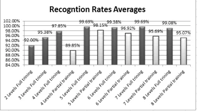
For the system based on wavelet methods the number of decomposition levels is the main parameter which affects the performance of the system, for the system based on HWT the optimal number of decomposition levels is five in which the EEG signal is decomposed in six-sub bands (Delta, Theta, Alpha, Gamma, and high Gamma) [7], as shown in Figures 5 and 6 when the system is fully and partially trained. The proposed system using Statistical Moments 2nd _{set that given by Eq. (15)}

on the HWT sub-bands was tested on CSU and MMI datasets and the full / partial training results for the both datasets are shown in Tables 6 and 7, respectively.

Figure 5: Recognition Rates averages versus the number of decomposition levels for HWT, CSU dataset

Figure 6: Recognition Rates averages versus the number of decomposition levels for HWT, MMI dataset

Table 6: Some achieved CRR results using Statistical moment’s 2nd _{set of HWT features and nMSD measure,}

CSU dataset

Full Training Partial Training Feat. Set CRR% Test set Train set Total result P4-Rotat 100% 95.24% 97.73% 96.92% P3-Rotat 98.46% 95.24% 100% 98.46% P4-Math 98.46% 80.95% 100% 93.85% C3-Rotat 98.46% 85.71% 93.18% 90.77% P4-Lett 98.44% 90.48% 95.35% 93.85% P3-Lett 98.44% 95.24 93.02 93.85% O2-Math 96.92% 85.71% 93.18% 90.77% C4-Lett 96.88% 80.95% 100% 93.85% C3-Baseline 95.38% 85.71% 95.45% 92.30%

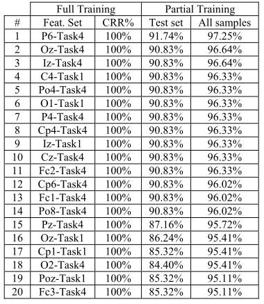
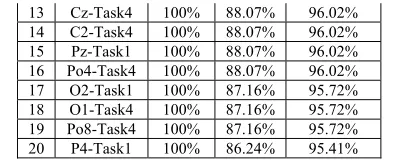
Table 7: CRR results using Statistical Moments 2nd _{set of}

HWT features and nMSD measure, MMI dataset Full Training Partial Training # Feat. Set CRR% Test set All samples 1 P6-Task4 100% 91.74% 97.25% 2 Oz-Task4 100% 90.83% 96.64% 3 Iz-Task4 100% 90.83% 96.64% 4 C4-Task1 100% 90.83% 96.33% 5 Po4-Task4 100% 90.83% 96.33% 6 O1-Task1 100% 90.83% 96.33% 7 P4-Task4 100% 90.83% 96.33% 8 Cp4-Task4 100% 90.83% 96.33% 9 Iz-Task1 100% 90.83% 96.33% 10 Cz-Task4 100% 90.83% 96.33% 11 Fc2-Task4 100% 90.83% 96.33% 12 Cp6-Task4 100% 90.83% 96.02% 13 Fc1-Task4 100% 90.83% 96.02% 14 Po8-Task4 100% 90.83% 96.02% 15 Pz-Task4 100% 87.16% 95.72% 16 Oz-Task1 100% 86.24% 95.41% 17 Cp1-Task1 100% 85.32% 95.41% 18 O2-Task4 100% 84.40% 95.41% 19 Poz-Task1 100% 85.32% 95.11% 20 Fc3-Task4 100% 85.32% 95.11%

d. Statistical Moments of Daubechies (db4) Sub-bands results

6123 shown in Figures 7 and 8 when the same conducted tests in HWT were applied.

Figure 8: Recognition Rates averages versus the number of decomposition levels for db4, MMI dataset

Table 8 shows some of full and partial training results of feature sets when db4 transform was applied and Statistical Moments 2nd _{set was}

used to extract the features of CSU dataset, while

Table 9 shows the result of MMI dataset when the

Statistical Moments 1st _{set was applied because it}

Achieved better results on MMI dataset than 2nd _set.

Figure 7: Recognition Rates averages versus the number of decomposition levels for db4, CSU dataset

Figure 8: Recognition Rates averages versus the number of decomposition levels for db4, MMI dataset

Table 8: Some achieved CRR results using Statistical Moments 2nd _{set of Daub4 features and nMSD measure,}

CSU dataset Full Training Partial Training

Feat. Set CRR% Test set Train set Total result O2-Rotat 100% 100% 100% 100% O2-Math 100% 95.24% 100% 98.46%

C3-Baseline 100% 95.24% 100% 98.46% P3-Rotat 98.46% 95.24% 100% 98.46% O1-Count 98.46% 95.24% 97.73% 96.92% P4-Rotat 100% 95.24% 97.73% 96.92% O1-Baseline 96.92% 85.71% 100% 95.38% C3-Lett 98.46% 85.71% 97.67% 93.85% P4-Math 96.92% 85.71% 97.67% 93.85% P3-Math 95.38% 85.71% 97.67% 93.85%

Table 9: Some achieved CRR results using Statistical Moments 1st _{set of Daub4 features and nMSD measure,}

MMI dataset

Full Training Partial Training # Feat. Set CRR% Test set Total result 1 Po4-Task4 100% 91.74% 97.55% 2 P6-Task4 100% 91.74% 97.25% 3 Iz-Task1 100% 90.83% 96.94% 4 Iz-Task4 100% 90.83% 96.64% 5 O1-Task1 100% 90.83% 96.33% 6 Cp4-Task4 100% 90.83% 96.33% 7 P4-Task4 100% 90.83% 96.33% 8 Fc2-Task4 100% 90.83% 96.33% 9 Oz-Task4 100% 90.83% 96.33% 10 Cz-Task4 100% 90.83% 96.33% 11 C4-Task1 100% 90.83% 96.33% 12 Fc1-Task4 100% 90.83% 96.02% 13 Pz-Task4 100% 87.16% 95.72% 14 O2-Task4 100% 86.24% 95.41% 15 Cp1-Task1 100% 86.24% 95.41% 16 Oz-Task1 100% 86.24% 95.41% 17 Cpz-Task1 100% 85.32% 95.11% 18 C3-Task4 100% 85.32% 95.11% 19 C2-Task4 100% 85.32% 95.11% 20 O1-Task4 100% 83.49% 94.50%

e.Statistical Moments Of Bi-Orthogonal (Tap9/7) Results

As the two previous wavelet methods the number of decomposition levels is the main parameter which affects the performance of the system that based on Tap 9/7, the optimal number of decomposition levels chosen was 5 as shown in Figures 9 and 10 when the same conducted tests were applied.

The best results of the identification system based on Statistical Moments of Bi-orthogonal (Tap9/7) Sub-bands are showed for CSU dataset using Statistical Moments 2nd _{set and for MMI}

dataset using Statistical Moments 1st _{set. Tables 10}

6124 Figure 9: Recognition Rates averages versus the number

of decomposition levels for Tap 9/7, CSU dataset

Figure 10: Recognition Rates averages versus the number of decomposition levels for db4, MMI dataset

Table 10: Some achieved CRR results using Statistical Moments 2nd _{Set of (Tap9/7) features and nMSD}

measure, CSU dataset Full Training Partial Training Feat. Set CRR% Test set Train set Total result

P4-Rot 100% 100% 97.73% 98.46% O2-Rot 100% 95.24% 100% 98.46% P3-Rot 98.46% 100% 97.73% 98.46% O1-Rot 96.92% 95.24% 97.73% 96.92% C3-Baseline 100% 85.71% 100% 95.38% C3-Comp 98.44% 85.71% 100% 95.38% P4-Comp 98.44% 95.24% 95.35% 95.31% O2-Multip 98.46% 90.48% 97.73% 95.31% P4-Baseline 96.92% 85.71% 100% 95.31% P4-Multip 98.46% 85.71% 100% 95.31%

Table 11: Some achieved CRR results using Statistical Moments Set1 of (Tap9/7) features and nMSD measure,

MMI dataset

Full Training Partial Training # Feat. Set CRR% Test set Total result 1 P4-Task4 100% 96.33% 98.78% 2 O2-Task4 100% 94.50% 98.17% 3 Oz-Task4 100% 93.58% 97.86% 4 P6-Task4 100% 92.66% 97.55% 5 Poz-Task4 100% 92.66% 97.55% 6 Pz-Task4 100% 92.66% 97.25% 7 P3-Task4 100% 90.83% 96.94% 8 Po4-Task1 100% 90.83% 96.94% 9 P2-Task4 100% 90.83% 96.64% 10 Po3-Task4 100% 90.83% 96.64% 11 Fc2-Task4 100% 88.99% 96.33% 12 Cp1-Task4 100% 88.99% 96.33%

13 Cz-Task4 100% 88.07% 96.02% 14 C2-Task4 100% 88.07% 96.02% 15 Pz-Task1 100% 88.07% 96.02% 16 Po4-Task4 100% 88.07% 96.02% 17 O2-Task1 100% 87.16% 95.72% 18 O1-Task4 100% 87.16% 95.72% 19 Po8-Task4 100% 87.16% 95.72% 20 P4-Task1 100% 86.24% 95.41%

3.2 Processing Time Results

To evaluate the performance of each recognition system the processing time is another important parameter; Tables 12 and 13 show comparisons of the average processing time for CSU dataset and MMI dataset respectively in milli-sec for each proposed method and comparing the results with our previous work which proposed in [24]. Taking into account the recording time for CSU dataset is (10 sec) with sampling rate (250 Hz), and the recoding time was taken for MMI CSU datasets (1 minute) and sampling rate is (160 Hz) and the matching time is for one-to-many comparisons. The Computer specification which we used was Intel® Core ™ i5-2450M CPU, with (4GB) RAM, operating system is windows7 (64bit), and the programming language was used is Microsoft visual C#.

Table 12: Comparisons of the average processing time results in msec for CSU dataset

Proposed Method

Feature

Extraction Matching Total DFT 13.359 0.013 13.372 DCT 22.0991 0.013 22.112 HWT 1.7495 0.014 1.763 Daub4 0.95797 0.014 0.972 Tap9/7 1.007 0.014 1.021

Table 13: Comparisons of the average processing time results in milli-sec for MMI dataset

Proposed Method

Feature

Extraction Matching Total DFT 217.364 0.13 217.494 DCT 323.864 0.17 324.034

HWT 3.559 0.16 3.719

Daub4 3.389 0.16 3.549 Tap9/7 3.719 0.16 3.879

4.COMPARISON WITH RECENTLY RELATED WORKS

6125 this article has low computational complexity and require very little execution time; also the system uses minimum number of channels(i.e. single channel) when subject applies certain single task.

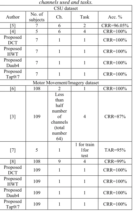
This comparison was conducted on system accuracy, taking in the consideration the number of electrodes used and the number of tasks performed by the test subjects to extract the discriminative features.

Table 14: The comparison with other published works on CSU dataset and MMI dataset based on Subjects number,

channels used and tasks. CSU dataset

Author _subjects No. of Ch. Task Acc. %

[5] 7 6 2 CRR=96.05%

[4] 5 6 4 CRR=100%

Proposed

DCT 7 1 1 CRR=100%

Proposed

HWT 7 1 1 CRR=100%

Proposed

Daub4 7 1 1 CRR=100%

Proposed

Tap9/7 7 1 1 CRR=100%

Motor Movement/Imagery dataset

[6] 108 2 1 CRR=100%

[3] 109

Less than half number

of channels

(total number

64)

4 CRR=87%

[7] 5 1

1 for train 1for

test TAR=95%

[8] 108 9 4 CRR=99%

Proposed

DCT 109 1 1 CRR=100%

Proposed

HWT 109 1 1 CRR=100%

Proposed

Daub4 109 1 1 CRR=100%

Proposed

Tap9/7 109 1 1 CRR=100%

The published works haven't mentioned the processing time clearly, so we can’t compare with them.

5.CONCLUSION AND FUTURE WORK

We investigated in this work multiple feature extraction methods and make a comparison among them. For each proposed method the system was fast, simple and achieved high results. The tests results indicated high performance for subjects' identification. The test results showed that

the proposed methods achieved perfect recognition rate (i.e., 100%) for identification when using minimum number of channels and tasks (i.e., one channel, single task) on CSU dataset an MM/IM dataset. DFT and DCT showed best recognition rates than wavelet based methods, but WT methods showed complexity and processing time less than others.

Another approach based on fusion of features from two channels belong to same task (i.e. two channels single task) can be explored to increase the degree of discrimination among subjects using the same above proposed methods.

REFERENCES:

[1] Marcos Del Pozo-Banos, Jesús B. Alonso, Jaime R. Ticay-Rivas, and Carlos M. Travieso, "Electroencephalogram subject identification: A review," Expert Systems with Applications, vol. 41, no. 15, pp. 6537-6554, 2014.

[2] Mohammed Abo-Zahhad, Sabah Mohammed Ahmed, and Sherif Nagib Abbas, "State-of-the-art methods and future perspectives for personal recognition based on electroencephalogram signals," IET Biometrics, vol. 4, no. 3, pp. 179–190, 2015.

[3] Douglas Rodrigues, Gabriel F.A. Silva, João P. Papa, and Aparecido N. Marana, "EEG-based person identification through binary flower pollination algorithm," Expert Systems with Applications, vol. 62, pp. 81-90, 2016.

[4] Ramaswamy Palaniappan, "Electroencephalogram signals from imagined activities: A novel biometric identifier for a small population," in International Conference on Intelligent Data Engineering and

Automated Learning, 2006, pp. 604-611.

[5] Pinki Kumari and Abhishek Vaish, "Feature-level fusion of mental task’s brain signal for an efficient identification system," Neural Computing and Applications, vol. 27, no. 3, pp. 659-669, 2015.

[6] D. La Rocca, P. Campisi, B. Vegso, P. Cserti, and G. Kozmann, "Human brain distinctiveness based on EEG spectral coherence connectivity," IEEE Transactions on Biomedical Engineering, vol. 61, no. 9, pp. 2406-2412, 2014.

[7] Pinki Kumari Sharma and Abhishek Vaish, "Individual identification based on neuro-signal using motor movement and imaginary cognitive process,"

Optik-International Journal for Light and Electron Optics,

vol. 127, no. 4, pp. 2143-2148, 2015.

6126 [9] Zachary A. Keirn and Jorge I. Aunon, "A new mode of

communication between man and his surroundings," IEEE transactions on biomedical engineering, vol. 37, no. 12, pp. 1209--1214}, 1990.

[10] _{Colorado State University Brain-Computer Interfaces}

Laboratory. (1989) [Online].

http://www.cs.colostate.edu/eeg/data/alleegdata.ascii.gz [11] Gerwin Schalk, Dennis J. McFarland , Thilo

Hinterberger, Niels Birbaumer, and Jonathan R.Wolpaw, "BCI2000: a general-purpose brain-computer interface (BCI) system," IEEE Transactions on biomedical engineering, vol. 51, no. 6, pp. 1034--1043, 2004.

[12] EEG Motor Movement/Imagery Dataset. [Online]. https://www.physionet.org/pn4/eegmmidb/

[13] Salahiddin Altahat, Michael Wagner, and Elisa Martinez Marroquin, "Robust electroencephalogram channel set for person authentication," in Acoustics, Speech and Signal Processing (ICASSP), 2015 IEEE International Conference on, vol. 997-1001, 2015. [14] Nasir Ahmed, T Natarajan, and Kamisetty R Rao,

"Discrete cosine transform," IEEE transactions on Computers, vol. 100, no. 1, pp. 90-93, 1974.

[15] Darius Birvinskas, Vacius Jusas, Ignas Martisius, and Robertas Damasevicius, "EEG dataset reduction and feature extraction using discrete cosine transform," in Computer Modeling and Simulation (EMS), 2012 Sixth

UKSim/AMSS European Symposium on, 2012, pp.

199-204.

[16] Asmaa M.J. Abbas and Loay E. George, "Palm Vein Identification and Verification System Based on Spatial Energy Distribution of Wavelet Sub-Bands," International Journal of Emerging Technology and Advanced Engineering, vol. 4, no. 5, pp. 727-734, may 2014.

[17] Radomir S.Stanković and Bogdan J.Falkowski, "The Haar wavelet transform: its status and achievements," Computers and Electrical Engineering, vol. 29, no. 1, pp. 25-44, 2003.

[18] James S Walker, A primer on wavelets and their scientific applications.: CRC press, 2008.

[19] _{Jianhong Shen and Gilbert Strang, "Asymptotics of} daubechies filters, scaling functions, and wavelets.,"

Applied and Computational Harmonic Analysis, vol. 5,

no. 3, pp. 312-331, 1998.

[20] Beladgham Mohammed, Bessaid Abdelhafid, Abdelmounaim Moulay Lakhdar, and Abdelmalik Taleb Ahmed, "Improving quality of medical image compression using biorthogonal CDF wavelet based on lifting scheme and SPIHT coding," Serbian Journal of Electrical Engineering, vol. 8, no. 2, pp. 163-179,

2011.

[21]Alex Pappachen James and Sima Dimitrijev, "Ranked selection of nearest discriminating features," Human-Centric Computing and Information Sciences, vol. 2, no. 1, pp. 1-14, 2012.

[22]Suhaila N. Mohammed and Loay E. George, "Subject Independent Facial Emotion Classification Using Geometric Based Features," Research Journal of

Applied Sciences, Engineering and Technology, vol.

11, no. 9, pp. 1030-1035, 2015.

[23]William K Pratt, Digital Image Processing.: A Wiley-Inter Science Publication, 2001.