AN EMPIRICAL EVALUATION FOR THE INTRUSION DETECTION FEATURES BASED ON MACHINE LEARNING AND FEATURE SELECTION METHODS

ISSN: 1992-8645 www.jatit.org E-ISSN: 1817-3195

6003

PROBABILISTIC MODEL OF ALLOCATION LAWS OF

EXPERIMENTAL DATA IN INFORMATION SYSTEMS

1_{YURI YURIEVICH GROMOV,} 2_{YURI VIKTOROVICH MININ,}

3_{OLGA GENNADEVNA IVANOVA,} 4_{ALEKSANDR GEORGIEVICH DIVIN,} 5_{HUDA LAFTA MAJEED}

1,2,3,4,5 _{Tambov State Technical University}

Sovetskaya Str., 106, Tambov, 392000, Russia

E-mail: 1_{[email protected],} 2_{[email protected],} 3_{[email protected],} 5_{[email protected]}

ABSTRACT

On the basis of the beta distributions of the 1st and 2nd kind were received probabilistic models of distribution laws, which allow to approximate wider class of distribution laws of experimental data, than the existing Pearson’s system of distributions. The method of identification parameters was developed of the generalized beta distribution using power, exponential and logarithmic moments.

Keywords: Information System, Experimental Data, Probability, Distribution Laws, Approximation.

1. INTRODUCTION

There is a view of the law of distribution assumed to be known in classical mathematical statistics and observing the results of its parameters assessed values. But usually pre-form of the distribution law is unknown and theoretical assumptions do not allow it to establish unequivocally. Also, processing of the experimental data does not allow to calculate accurately true distribution law. In this case, you should talk only about the approximation (approximate description) of real law to some others which is consistent with experimental data and in some ways similar to the unknown true law.

Nowadays, for the approximation of the experimental data distribution laws often used Pearson distributions [1-26]. However, the determination of the parameters of the desired distribution from the family of Pearson distributions connected with the decision of the various systems of equations using the method of moments. Besides, the method of moments does not allow to find the parameter estimates those distributions, including those owned by the Pearson family which do not have higher order moments (3rd and 4th). That is why the development of continuous distributions systems wider than the family of Pearson curves, as well as new methods for estimating the parameters has great importance both in theoretical and applied research.

Except of the method of Pearson for this purpose can be used the method based on obtaining a new distribution as a random function argument with the known distribution [2,6,8].

2. STATEMENT OF THE PROBLEM

The main objectives of the work:

1) To receive generalized beta distribution based on the beta distribution of the 1st and 2nd kind using method of functional transformation.

2) To consider the possibility of approximating the distribution law of experimental data, taking positive and negative values or only positive values using generalized beta distribution of the 1st and 2nd kind.

3. SOLUTION OF THE PROBLEM

3.1 Unilateral Generalized Beta Distributions Of 1st And 2nd Kind

Probability density functions (PDF) for the classical beta distributions of 1st and 2nd kind are as follows [2,27]:



 



1

1 1 , )

( 





 _y v

v B

y y p





, 0<y<1; (1)

 

 







  _

v

y v B

y y

p _



, 1 1

, 0 <y< , (2)

6004 After a functional conversion yxc c or

c c _x

y PDF (1) respectively, we have





1 1

1 ,

) (

 

    

  

 

v

c c

c

c _x

v B

x c x p

 

 



, 0 <x<; (3)

 

 

1 1 1

,



 

     

 

v

c c

c c

x x

v B

c x

p 

 

 

,<x<, (4)

where  0, v 0, c 0 - parameters of the form; 

0 - scale parameter.

Specific cases of distribution (3) there is the power law when c = 1 и v = 1; Beta distribution when c = 1. The limiting case of (3) is a lognormal distribution when , v and c 0.A special case of PDF (4) is a Pareto distribution when c = 1 and v = 1 [27-29].

Using PDF (3) or PDF (4) and the ratio [30]





 0

) (x dx p x

m s

s , (5)

We can get the initial moments of s-th order for distributions (3)and (4)



 



  

v sc



v c

s m

s

s _{   }

    

 

 



;



 



  

v sc



v c

s m

s

s _{   }

    

 

 



, (6)

where



 

z

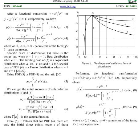
- is the gamma function.

From (6) it follows that for PDF (4), there are only the initial direct points, order s of those satisfies the condition s<c. On the image 1 are presented the regions of existence of PDF(3) and PDF(4) in the plane of variables K₁ and K₂, determined by the expressions (whenc1) [31]





.

; ₂

1 2 2

2 2 3 1 2 2

2 1 1

c c c

c c c

c c

m m m

m m m K m

m K

  

 (7)

On the image 1 the region of distribution’s existence (3) and it is special cases left to the curve 3, characterizing a region of existence of the standard logarithmic distribution. Curve 1 characterizes the region of existence of the power law, and the point G - Gaussian distribution. The region of existence of the beta distribution is located to the left of the curve 2.The region of existence of distribution (4) and its special cases is located to the right of the curve 3. The curve 5 characterizes the region of the existence of Pareto distribution.

0 0.5 1 1.5 2 2.5 3 3.5 4 0

0.2 0.4 0.6 0.8 1

K 2

K 1 _G

1 2

3 5

[image:2.612.78.526.58.469.2]

4

Figure 1. The diagram of unilateral laws of distribution

Performing the functional transformation c

c x

y  oryc xcof PDF (2), respectively obtain

 

 



       



  _v

c c c

c

x v

B

x c x

p _

 







, 1

1

, 0 <x<, (8)

 

 



    

  



 _



v

c c c

c

x x

v B

c x

p _

 

 



1

, 1

,0<x<, (9)

where v 0, 0 <≤v, c 0 - parameters of the form;

 0 –scale parameter.

Special cases of PRV (8) are: beta distribution of II sort with c = 1;F- distribution when  0,5n1,

2 5 ,

0 n

v , c = 1 andn₂ n₁[27].

After substituting the PDF (8) or PDF (9) in (5) and integration we obtain the early moments of s-th order for these distributions [32]



 



   

v

c s v c s m

s

s _{ }

    

  

. (10)



 



   

v c s v c s m

s

s _{ }

  

 

  

. (11)

From (10) it follows that for PDF (8), there are only the initial moments, order of which s satisfies the condition s<vс. From (11) it follows that there are only the starting points for the PDF (9)order of which s satisfies the conditions<c.

ISSN: 1992-8645 www.jatit.org E-ISSN: 1817-3195

6005

 

 

_       

 

c c

c

c _x

x c x p

 

 



exp 1

, 0<x<, (12)

where 0, c 0 –parameters of the form;  0 – scale parameter.

Special cases of (12) are: Rayleigh PDF when = 1,  2 and с = 2; exponential distribution with  = 1 and c = 1; gamma distribution when = v + 1,c = 1; chi-square distribution when = 0,5n, c= 1 и = 2; Nakagami distribution when = m,

m

 

 и c = 2; Weibull distribution when  = 1 andc= . Extreme cases (9) are the power law when  0 and c; lognormal distribution when

 and c 0 [5-7].

Substituting the (12) into (5) and integrating [28] we obtain the initial moments of the s-th order





 

  

  

 sc

m_s s . (13)

It should be noted, that the property, inherent in the distribution of (12) and presented in the form of equity [27]:



1





_{2 1} 2



1,

2 1

) 1

( _

 





c c c n

c c n c c n

m m m n

m m m m

(14)

when n 2. This property is proved by substituting expression (13) into (14) for the corresponding initial moments.

On the image 1the existence region of PRV (12) is located between the curves 1 and 3. Direct line 2 corresponds to the region of existence of the gamma distribution. The region of existence PDF(8) is located between curve 1 and curve 3. It is overlapped considerably with the region of existence of PDF (3) and includes a full region of existence of distribution (12).

Let’s consider the limiting case of PRVDF (4) and PDF (9) when the parameter v . In this case distributions (4) and (9) are converted into distribution

 

 

_       

 _

c c

c c

x x

c x

p 

 

 

exp

1 , 0<x<. (15)

where α 0, c 0 – parameters of the form;  0 – scale parameter.

Special cases of (15) when c = 1 V is a type of distribution of the Pearson classification, and when

с - is a Pareto distribution [27, 28]. Substituting the (15) in (5) and integrating, we obtain the initial moments of s-th order





  



   

 s c

m s

s . (16)

From (16) it follows that for the PRV (15), there are only the initial straight times, the order of which satisfies the condition s<c.

On the image 1 the existence region of PDF (15) is located between curves 3 and 5. The curve 4 describes a region of existence V-thtype distribution of the Pearson classification. The region of existence of distribution (9) is located between the third curve and the fifth curve. It is overlapped considerably with the region of the existence of distribution (4) and includes a full region of existence of PDF (15).

For the obtained distributions (3), (8) and (12) are characterized by two properties:

1) the property of moments defined by the equation:







3



1

4

4 3

3 2 1 1 2 2

2 2 3 1 1 3 2 4

3 _

 

 



c c c c c

c c c c c c c c

m m m m m

m m m m m m m

m _{. (17)}

2) The condition of distribution (3)isK₂ 1, for distributing (12) - K₂ 1and for distributing (8) -

1 2 

K .

These properties are also valid for the distribution (4), (9) and (15), if to substitute in relations (7) and (17) instead of direct power moments inverse points. In this case for distribution (4) is still the conditionK₂ 1, for distributing (15) - K₂ 1and for distributing (9) -K₂ 1.These properties can be used to identify the generalized beta distribution.

Let us to consider now the limiting cases for generalized beta distribution of the 1st and 2nd kind, when the parameter с 0. In this case distribution (12) and (15) are converted into logarithmic normal distribution. The expression for the PDF has the form





    

 

 _

 

2 2 2

) ln( exp 2

1 ) (

  



x x

x

p , (18)

where  0,  0 - distribution options.

For the distribution of (18) there are all direct and inverse power moments. Therefore PDF parameters are defined by the first initial and the second central moments of the logarithmic

2 1, ˆ ˆ

ˆ

ˆl   L

 . (19) The region of existence PRV (18) is shown at the image 1 by the curve 3.

Distribution (3) and (8) converted into distribution, when the parameter с 0

1 1

ln ) ( ) (

 

     

      



v v

x v

x x

p 

 

 

6006 where v> 0, β> 0 – parameters of the form; χ> 0 – scale parameter.

Substituting the PDV (20) in equation (5) and integrating [32], we get the early moments of the s-th order









v s

s s

m     . (21) On the image 1 the existence region of distribution (20) is located to the left of the curve 3.

When с0 distributions (4) and (9) are converted into distribution

1 1 ln

) ( ) (



 

    

      



v

v _x

x v x p

 



 

, χ<x<, (22)

where v> 0, β> 0 – parameters of the form; χ> 0 – scale parameter.

Substituting the GHD (22) into (5) and integrating [32], We obtain the initial moments of s-th order









v s

s s

m     . (23) From (23) it follows that for distributing (22) there are all inverse initial moments and only those points straight, order of which satisfies s. On the image 1 the region of distribution’s existence (22) is located to the right of the curve 3. The distribution parameters (22) are defined by (23) with the help of reverse moments.

Identification of the lognormal distribution (18) is possible only with the use of logarithmic points [27]. Except of PDF (18), this group includes the distribution





_{1 2} 1

ln ln ) , 5 , 0 (

) ln( 5 , 0 ) (

 

   

 

            



v v

x h

x x v B

h x

p 

 ,hχ<x<χ; (24)

 







₂





₂



0,5 2

) ln( ,

5 ,

0   

 v _v

x x

v B x p







,0<x<. (25)

where 0<h< 1–the form parameter.

They are also limiting distributions for generalized beta distribution. There is only a portion of the logarithmic moments existing for PDF (25). Thus, we get a wide class of models of unilateral laws of distributions based on beta-distributions of the 1st and 2nd kind. When we identifying generalized beta distribution taking into account the consideration of their properties, you can use the forward and reverse power moments (including fractional order), and logarithmic moments [31,33,34].

3.2 Identification Of Unilateral Generalized Beta Distributions Of The 1st And 2nd Kind

Approximation of the experimental distributions with the help of unilateral generalized beta

distribution can be carried out using the following algorithm:

1. Initially are determining logarithmic sampling points





 n

i i

x n l

1 1 1 ln



,











 n

i

s i

s _n x l

L

1

1 ) ln(

1 



, s = 2, 3, (26)

and then an estimate the asymmetry coefficient

5 , 1 2 3

L

L

L



_a







.

2. If for the coefficient

L



_a the following

condition is



0

,

1



L

a



0

,

1



, then further defined selective central point

L



₄and is a joint evaluation of coefficient skewness and kurtosis

2 2 4

2 2

3

6

L

L

L

L

_ae

_

_









_.

When the condition

L



_ae> 1,04to approximate of the experimental distribution is used the distribution (24) with parameters

; 1 5 , 1 ˆ

  

ae ae

L L

v _



; 1

2 exp

ˆ _{2 1}

  

  

  

 L l

L L

ae

ae  

 



    

  

  

 2

1 2 2 exp

ˆ _L

L L h

ae ae 

 

.

If for the coefficient La



the following condition is 0,96L_ae 1,04, the lognormal distribution (22) is used to approximate the experimental distribution, whose parameters according to (23) defined by the initial first and second central logarithmic moments (ˆl₁,ˆ L₂ ).

When the condition

L



_ae< 0,96to approximate the experimental distribution is used the distribution (25) with parameters

1 2 ; ˆ 1

2 ˆ ; 1

5 , 1 2

ˆ L l

L L L

L v

ae ae

ae

ae  

  



 

  



   .

ISSN: 1992-8645 www.jatit.org E-ISSN: 1817-3195

6007 determined as follows: first estimate is the parameter c of the solution of equation







3ˆ ˆ ˆ



1

ˆ ˆ 4 ˆ ˆ ˆ 4 ˆ ˆ ˆ 3 ˆ ˆ 3 2 1 1 2 2 2 2 3 1 1 3 2 4 3 _      c c c c c c c c c c c c c m m m m m m m m m m m m m

, (27)

where



  n i c i

c _n x

m 1 1 1   _,

_

  n i c i

c _n x

m 1 2 2 1   _,



  n i c i c x n m 1 3 3 1   _,

_

  n i c i c x n m 1 4 4 1 

 _{. (28)}

Then, the coefficient’s estimates are determined as K₁иK₂with help of the relations (7). If the conditionKˆ2 1, thenfor the approximation of the

experimental distribution, use distribution (3) with parameters ; ˆ ˆ 2 ˆ 1 ˆ ˆ 2 ˆ 2 1 2 2 1 K K K K K     c c v m K K v ˆ 1 1 2 2 ˆ ˆ 1 ˆ ˆ ; ˆ ˆ 1 ˆ 2 ˆ _                  

 . (29)

If Kˆ₂ 1, then to approximate the experimental distribution is used the distribution (12) with parameters

c c

m K

K ₁ 1ˆ

1 1 ˆ ˆ ˆ ; ˆ 1 ˆ ˆ _          

 . (30)

When the condition isKˆ2 1to approximate the

experimental distribution is used the distribution (8) with the following parameters

; ˆ ˆ 2 ˆ 1 ˆ ˆ 2 ˆ 2 1 2 2 1 K K K K K     c c v m K K v ˆ 1 1 2 2 ˆ 1 ˆ ˆ ˆ ; 1 1 ˆ ˆ 2 ˆ            

 . (31)

4. If the ratio L_a> 0,1, then for the approximation of the experimental distribution is used one of the distributions (4), (9) or (15).Type of distribution and its parameters can be determined as follows: first evaluate determined parameter c by solving the equation (27), and then determine the coefficient’s estimates K₁ и K₂ with help of the relations (7). In this case, relations (7) and (17) are now used selective inverse points



   n i c i c x n m 1 1 1   _,

_

   n i c i c x n m 1 2 2 1   _,



   n i c i c x n m 1 3 3 1   _,

_

   n i c i c x n m 1 4 4 1 

 _{. (32)}

If the condition Kˆ2 1, you should use the

distribution (4) for the approximation of the experimental distribution with parametersˆ ,

v

andˆ, which are defined by (29) with considering the (32).

IfKˆ2 1, then to approximate the experimental

distribution the distribution (15)with parameters

ˆ andˆ_{are used, defining relations (30) with}

considering the (32).

When the condition Kˆ2 1is true for

approximating the experimental distribution is used the distribution (9) with parameters (31)

5. When the parameter’s estimatecˆ → 0 (on practice cˆ ≤ 0,1), then the approximation of the experimental distributions is made with distributions (20) and (22). If the ratio L_a< - 0,1, It is used PDF (20) to approximate the distribution. Its parameters can be determined as follows: first find the estimate of the parameter β is determined by solving the equation

 

 

 

2ln

     

ˆ

   

1 ln ˆ ln ˆ 2 ˆ 1 1 ˆ ln ˆ ln ˆ ln 2 ˆ ln ˆ ˆ ln 1 2 1 1                 m m l m , where



  n i i x n m 1 1 1  _,

_

  n i i x n m 1 2 2 1  _.

Then, evaluation parameters are v and  determined with the aid of relations

 

   

ˆ _lnˆ _{1 1} ˆ ln

ˆ ˆ ln

ˆ 1 1

  



 m l

v , _

          ˆ ˆ ˆ exp

ˆ l₁ v .

If the ratios L_a> 0,1and cˆ ≤ 0,1, then is used PDF (22) for approximating the distribution. It’s parameters are defined in a similar distribution of parameters (20). The estimate of parameter  is determined by solving the equation

 

 

 

2ln

     

ˆ

   

1 ln ˆ ln ˆ 2 ˆ 1 1 ˆ ln ˆ ln ˆ ln 2 ˆ ln ˆ ˆ ln 1 2 1 1                 m m l m , where



  n

i xi

n m

1

1 1 1

 _,

_



 n

i xi

n m

1 2

2 1 1

 _.

Parameter’s estimates v and  corresponding expression

 

   

ˆ _lnˆ _{1 1} ˆ ln

ˆ ˆ ln

ˆ 1 1

  



 m l

v , _

          ˆ ˆ ˆ exp

6008 If the resulting parameter estimate cˆ 3, it can  be assumed that cˆ 3. The error of approximation 

of the experimental distribution increases slightly. Our procedure approximation of the experimental distributions should be used when sample size ofn1000.

Similarly it is possible to carry out an approximation of the theoretical distributions, but instead of the sample moments in this case use the appropriate power and logarithmic points of approximating the theoretical distribution.

3.3 Bilateral Generalized Beta Distribution And Their Identification

Bilateral generalized beta distribution can be obtained by functional transformation zln(x)

unilateral generalized beta distribution of the 1st and 2nd kind. As a result, the functional transformation of the distributions (3), (4), (8), (9), (12), (15), (18), (20), (22), (24) and (25) will take correspondingly the following form:

 





 

,



1 exp



 





1 exp

)

(    _cz v

v B

z c c z

p 

  

,-∞<z<μ;(33)









 

,



1 exp











1 exp

)

(     _{c z} v

v B

z c c

z

p 

  

μ<z< ∞;

(34)

 









 





















 _

v

z c v

B

z c c z

p _

 

  exp 1 ,

exp

, - <z<;(35)

 









 





















 

 _

v

z c v

B

z c c

z

p _

 

  exp 1 ,

exp

, - <z<;(36)

 



_{ }





















  

  



c cz cz

z

p exp exp exp ,-<z<;(37)

 



_{ }





















  

   

 

c cz cz

z

p exp exp exp

- <z<;

(38)

 





, z ;

2 exp 2

1

2 2

         

 

 _

 

  



z z

p (39)

    

 1exp













, - z ;



 _  _{   }



 _z  _z

z

p (40)

    

 1exp













, z;



 _  _{  }



 _z  _z

z

p (41)

  

_{ }

 

_{ }



    



   





    

   

 z _ z  x

z p

v

, , 5 . 0 1 2

1 1

; (42)

 







₂





₂



0,5 2

, 5 ,

0   

 v _v

z v B z p







, - <z<;(43)

where - shift parameter. In (35) and (36) satisfies the condition 0 <≤ v.

Bilateral generalized beta distribution of the 1st and 2nd kind (33)-(43) can be used for the approximation of the experimental distributions NE, taking negative and positive values. When defining their parameters instead of random direct and inverse power moments using direct and inverse exponential moments, and selective direct power points instead of logarithmic moments. This allows you to apply for identification of the parameters of bilateral generalized beta distribution algorithm, discussed above in Section 2. It is found that if the ratio La< 0, then in the law of distribution are dominating direct exponential moments, and if La> 0, the predominant circulating exponential moments. Similarly it is possible to carry out an approximation of the theoretical distributions of bilateral, but instead of sampling points used in this case the corresponding power and exponential moments approximating the theoretical distribution are used.

4. CONCLUSIONS

Thus, there were proposed generalized beta distribution to approximate the laws of unilateral and bilateral distribution of experimental data. This allows to receive wider class of distributions laws, than the existing system of Pearson distributions. Was developed a method for identifying the parameters of generalized beta distribution of the 1st and 2nd kind with the use of power, exponential and logarithmic moments. In this case it is possible in many cases to increase the accuracy of the parameter’s estimates of the distributions. A topographic classification of unilateral distribution laws was developed.

The work was supported by the Ministry of Education and Science of the Russian Federation under the Agreement No 14.577.21.0214 (identifier RFMEFI57716X0214).

REFRENCES:

[1] Pearson K. On the dissection of asymmetrical frequency curves // Phil. Trans. Roy. Soc. – 1894, Vol. A185. Pp. 71-110.

[2] Kendall M., Stjuart A. Teorija raspredelenij [Theory of distributions] - M.: Nauka, 1966. (Rus).

rabot-ISSN: 1992-8645 www.jatit.org E-ISSN: 1817-3195

6009 nikov [Applied mathematical statistics. For engineers and scientists] - M.: Fizmatlit, 2006. (Rus).

[4] Gromov Yu.Yu., Karpov I.G. Zakony raspredelenija nepreryvnoj sluchajnoj velichiny s maksimal'noj jentropiej. Obobshhennyj metod momentov [Laws of distribution of continuous random variable with maximum entropy. Generalized Method of Moments] // Nauchno-tehnicheskie vedomosti Sankt-Peterburgskogo gosudarstvennogo politehnicheskogo universiteta. Informatika. Telekommunikacii. Upravlenie. 2009. Vol. 1. No 72. Pp. 37-42. (Rus)

[5] [5] Karpov I.G., Gromov Yu.Yu., Samharadze T.G. Approksimacii raspredelenij konechnoj summy nepreryvnyh sluchajnyh velichin [Approximations of distributions of a finite sum of continuous random variables] // Inzhenernaja fizika. 2009. No 3. Pp.28-31. (Rus)

[6] [6] Gromov Yu.Yu., Karpov I.G. Dal'nejshee razvitie sushhestvujushhih predstavlenij ob osnovnyh formah zakonov raspredelenij i chislovyh harakteristik sluchajnyh velichin dlja reshenija zadach informacionnoj bezopasnosti [Further development of existing ideas about the basic forms of distribution laws and numerical characteristics of random variables for solving problems of information security] // Informacija i bezopasnost'. 2010. Vol. 13. No 3. Pp. 459-462. (Rus)

[7] [7] Gromov Yu.Yu., Karpov I.G., Nurutdinov G.N. Postroenie zakonov raspredelenija s mak-simal'noj jentropiej dlja ocenki riskov v informacionnyh sistemah [Construction of distribution laws with maximum entropy for risk assessment in information systems] // Informacija i bezopasnost'. 2011. T.14. No 3. Pp.447-450. (Rus)

[8] [8] Bostandzhijan V.A. Raspredelenie Pirsona, Dzhonsona, Vejbulla i obratnoe normal'noe. Ocenivanie ih parametrov [The distribution of Pearson, Johnson, Weibull and the inverse of the normal. Estimation of their parameters]- Chernogolovka: Redakcionno-izdatel'skij otdel IPHF RAN, 2009. (Rus)

[9] [9] Gromov Yu.Yu., Denisov A.P., Matveykin V.G. Modelirovanie i upravlenie slozhnymi tehnicheskimi sistemami [Modeling and management of complex technical systems]. - Tambov: TSTU, 2000. - 291 p. (Rus).

[10][10] Gromov Yu.Yu., Denisov AP, Matveykin V.G. Voprosy modelirovanija i upravlenija slozhnoj transportnoj sistemoj [The problems

of modeling and managing a complex transport system]. - Moscow: Mechanical Engineering-1, 2002. - 291 p. (Rus).

[11]Gromov Yu.Yu., Drachev V.O., Nabatov K.A., Ivanova O.G. Sintez i analiz zhivuchesti setevyh sistem [Synthesis and analysis of the survivability of network systems]. - Moscow: Mechanical Engineering-1, 2007. - 150 c. [12]Nabatov K.A ., Gromov Yu. Yu .; Kalinin

V.F., Serbulov Yu.S., Drachev V.O. Raspredelenie resursov setevyh jelektrotehnicheskih sistem [Distribution of resources of network electrical systems]. - Moscow: Mechanical Engineering, 2008. - 238 p. (Rus).

[13]Ischuk I.N., Fesenko A.I., Gromov Yu.Yu. Identifikacija svojstv skrytyh podpoverhnostnyh ob#ektov v infrakrasnom diapazone voln [Identification of the properties of hidden subsurface objects in the infrared range of waves]. - Moscow: Mechanical Engineering, 2008. - 182 c. (Rus). [14]Gromov Yu.Yu. Mishchenko S.V., Pogonin

V.A., Nabatov K.A. Jenergosberegajushhie informacionno-upravljajushhie sistemy ob#ektami maloj jenergetiki [Energy-saving information and control systems of small power engineering objects]. - Moscow: Nauchtehlitizdat, 2010. - 202 p. (Rus).

[15]Alekseev V. V., Gromov Yu. Yu., Yakovlev A. V., Starozhilov O. G. Analiz i sintez modul'nyh setevyh informacionnyh sistem v interesah povyshenija jeffektivnosti celenapravlennyh processov [Analysis and synthesis of modular network information systems in the interests of increasing the efficiency of purposeful processes]. - Tambov [and others]: Nobelistics, 2012. - 130 p. (Rus).

[16]Gromov Yu.Yu., Ivanovskiy M.A., Didrikh V.E., Ivanova O.G. Martemyanov Yu.F. Metody analiza informacionnyh sistem [Methods of analysis of information systems]. - Tambov [and others]: Nobelistics, 2012. - 219 p. (Rus).

6010 [18]Voronov I.V. Primenenie universal'nogo

semejstva raspredelenij Pirsona dlja approksimacii raspredelenija znachenij vektora psevdogradienta pri sovmeshhenii izobrazhenij [Application of the universal family of Pearson distributions for approximating the distribution of values of the pseudogradient vector when images are combined] // Radiojelektronnaja tehnika. - 2015. - No. 2 (8). - P. 123-127. (Rus).

[19]Bostandzhyan B.A. Raspredelenie Pirsona, Dzhonsona, Vejbulla i obratnoe normal'noe. Ocenivanie ih parametrov [The distribution of Pearson, Johnson, Weibull and the inverse of the normal. Estimation of their parameters]. - Chernogolovka: Redakcionno-izdatel'skij otdel IPHF RAN, 2009. - 240 p. (Rus).

[20]Sukhanov VI, Timoshenko S.I., Chernin R.M. Issledovanie vizualizacii dannyh s primeneniem otkrytyh geoinformacionnyh servisov [Investigation of data visualization using open geoinformation services] // Informacionnye sistemy i tehnologii. - 2011. - No. 6 (68). - P. 139-144.

[21]Timoshenko, S.I. Ispol'zovanie semejstv krivyh Dzhonsona i Pirsona v zadachah approksimacii raspredelenij, rascheta i ocenki verojatnostnyh harakteristik [Using families of Johnson and Pearson curves in problems of approximating distributions, calculating and estimating probabilistic characteristics] // UPI. - Sverdlovsk, 1986. - 59 p. (Rus).

[22]Bityukova V.V., Khvostov A.A., Rebrikov D.I. Primenenie universal'nyh semejstv raspredelenij Pirsona dlja modelirovanija zagruzhennosti kabinetov lechebno-profilakticheskih uchrezhdenij [Application of universal families of Pearson distributions for modeling the workload of the cabinets of medical and preventive institutions] // Vestnik

Tambovskogo gosudarstvennogo

tehnicheskogo universiteta [Bulletin of Tambov State Technical University]. - 2008. - T. 14, No. 1. - P. 202-208. (Rus).

[23]Chaudhry, M. A., Ahmad M. On a probability function useful in size modeling // Canadian Journal of Forest Research. 23. 1993. Pp.1679-1683.

[24]Dunning, K., Hanson, J. N. Generalized Pearson distributions and nonlinear programming // Journal of Statistical Computation and Simulation, 6, 1977. Pp. 115-128

[25]Lahcene B. On Pearson families of distributions and its applications // African

Journal of Mathematics and Computer Science Research. -Vol. 6(5). - May 2013. - pp. 108-117. DOI: 10.5897/AJMCSR2013.0465 [26]Mohammad Shakil, B. M. Golam Kibria, Jai

Narain Singh A New Family of Distributions Based on the Generalized Pearson Differential Equation with Some Applications // Austrian Journal Of Statistics, Volume 39 (2010), Number 3, Pp.259–278.

[27]Vadzinskij R.N. Spravochnik po verojatnostnym raspredelenijam [Handbook of probability distributions] – SPb.: Nauka, 2001. (Rus).

[28]Odnomernye nepreryvnye raspredelenija: chast' 1 [One-dimensional continuous distributions: part 1] / N.L. Dzhonson, S. Koc, N. Balak-rishnan. – M.: BINOM. Laboratorija znanij, 2010. (Rus)

[29]Odnomernye nepreryvnye raspredelenija: chast' 2 [One-dimensional continuous distributions: part 2] / N.L. Dzhonson, S. Koc, N. Balak-rishnan. – M.: BINOM. Laboratorija znanij, 2012. (Rus).

[30]Gnedenko B.V. Kurs teorii vepojatnostej [Course theory of vepoyatnost] – M.: Nauka, 1988. (Rus).

[31]Metody obobshhennogo verojatnostnogo opisanija i identifikacii negaussovskih slu-chajnyh velichin i processov [Methods of generalized probabilistic description and identification of non-Gaussian random variables and processes] / I.G. Karpov, M.G. Karpov, D.K. Proskurin – Voronezh: VGU, 2010. (Rus).

[32]Prudnikov A. P., Brychkov Ju. A., Marichev O.I. Integraly i rjady. Jelementarnye funkcii [Integrals and series. Elementary functions]. - M.: Nauka, 1984. (Rus).

[33]Karpov I.G. Priblizhennaja identifikacija zakonov raspredelenija pomeh v adaptivnyh priemnikah s ispol'zovaniem metoda momentov [Approximate identification of the laws of distribution of interference in adaptive receivers using the method of moments] // Radiotehnika. – 1998. No 3. Pp. 11-14. (Rus). [34]Karpov I.G., Evseev V.V. Approksimacija