BIROn - Birkbeck Institutional Research Online
Anastasiadis, A.D. and Magoulas, George D. and Vrahatis, M.N. (2006)
Improved sign-based learning algorithm derived by the composite nonlinear
Jacobi process. Journal of Computational and Applied Mathematics 191 (2),
pp. 166-178. ISSN 0377-0427.
Downloaded from:
Usage Guidelines:
Please refer to usage guidelines at or alternatively
Birkbeck ePrints: an open access repository of the
research output of Birkbeck College
http://eprints.bbk.ac.uk
Anastasiadis, Aristoklis D.; Magoulas, George D.
and Vrahatis, Michael N. (2006). Improved
sign-based learning algorithm derived by the composite
nonlinear Jacobi process.
Journal of Computational
and Applied Mathematics
191
(2) 166-178.
This is an author-produced version of a paper published in Journal of
Computational and Applied Mathematics (ISSN 0377-0427). This version has
been peer-reviewed but does not include the final publisher proof corrections, published layout or pagination.
All articles available through Birkbeck ePrints are protected by intellectual property law, including copyright law. Any use made of the contents should comply with the relevant law. Copyright © 2006 Elsevier B.V.
Citation for this version:
Anastasiadis, Aristoklis D.; Magoulas, George D. and Vrahatis, Michael N. (2006). Improved sign-based learning algorithm derived by the composite nonlinear Jacobi process.London: Birkbeck ePrints. Available at:
http://eprints.bbk.ac.uk/archive/00000501
Citation for the publisher’s version:
Anastasiadis, Aristoklis D.; Magoulas, George D. and Vrahatis, Michael N. (2006). Improved sign-based learning algorithm derived by the composite nonlinear Jacobi process. Journal of Computational and Applied Mathematics 191(2) 166-178.
Improved sign–based learning algorithm
derived by the composite nonlinear Jacobi
process
Aristoklis D. Anastasiadis
∗
School of Computer Science and Information Systems, Birkbeck College, University of London, London Knowledge Lab, 23-29 Emerald Street, WC1N 3QS,
London, United Kingdom.
George D. Magoulas
School of Computer Science and Information Systems, Birkbeck College, University of London, Malet Street, London WC1E 7HX, United Kingdom.
Michael N. Vrahatis
Computational Intelligence Laboratory (CI Lab), Department of Mathematics, University of Patras Artificial Intelligence Research Center (UPAIRC),
University of Patras, GR-26110 Patras, Greece.
Abstract
In this paper a globally convergent first–order training algorithm is proposed that uses sign–based information of the batch error measure in the framework of the nonlinear Jacobi process. This approach allows us to equip the recently proposed Jacobi–Rprop method with the global convergence property, i.e. convergence to a local minimiser from any initial starting point. We also propose a strategy that ensures the search direction of the globally convergent Jacobi–Rprop is a descent one. The behaviour of the algorithm is empirically investigated in eight benchmark problems. Simulation results verify that there are indeed improvements on the con-vergence success of the algorithm.
Key words: Supervised learning, nonlinear iterative methods, nonlinear Jacobi,
pattern classification, feedforward neural networks, convergence analysis, global convergence.
1 Introduction
Nowadays, artificial neural networks are vital components of many systems and are considered powerful tool for pattern classification [5,11]. The vast ma-jority of artificial neural network solutions have been trained with supervision.
In this context, the training phase is one of the most important stages for the neural network to function properly and achieve good performance. In supervised learning the desired outputs are supplied by a “teacher” and the network is being forced into producing the correct outputs by adjusting the weights iteratively, in order to globally minimize a measure of the difference between its actual output and the desired output for all examples in a training set [10]. Finding the global minimum is a difficult task in neural networks due to their complex objective functions, the so–called error function [10,27].
Back-Propagation (BP) [27] is a popular training algorithm, which minimizes
the error function by updating the weights w using the steepest descent
method [4]:
wk+1 =wk−η∇E(wk), k = 0,1,2, . . . (1)
whereE is thebatch error measuredefined as the Sum–of–Squared–differences
Error function (SSE) over the entire training set, while ∇E denotes the
gra-dient ofE. The parameter η is a heuristic, called step–size.
Choosing the right value for the step–size is very important as it has an impact on the training speed, the success of the learning process and the quality of the results produced by the network. First–order algorithms with individual adaptive step–sizes provide dynamic tuning of the step–size using adaptation techniques that are able to handle the trade off between maximising the length of the step–size and reducing oscillations [16,17]. A variety of approaches that use second derivative related information to accelerate the learning process have been proposed for small to medium size networks [4,15,18,33].
An inherent difficulty with first–order and second–order learning schemes is convergence to local minima. While some local minima can provide acceptable solutions, they often result in poor network performance. This problem can be overcome through the use of global optimization at the expense of an increase in the computational cost, particularly for large networks [7,21,22,30].
takes into account only the sign of the derivative to indicate the direction of the weight update. The effectiveness of Rprop in practical applications has motivated the development of several variants with the aim to improve the convergence behavior and effectiveness of the original method. Recently a mod-ification of the Rprop, the so–called Jacobi–Rprop (JRprop) method has been proposed [2,3]. Empirical evaluations of JRprop gave good results, showing that JRprop outperforms in several cases the Rprop and Conjugate Gradi-ent algorithms [3]. This paper proposes a globally convergGradi-ent JRprop-based learning scheme and derives a theoretical justification for its development.
This paper is organized as follows. First, we give a brief outline of the theoret-ical background behind the Jacobi–Rprop algorithm. Next, the new globally convergent algorithms is presented and a theoretical result that justifies its convergence is derived. Then we conduct an empirical evaluation of the new algorithm by comparing it with the classic Rprop, and the recently proposed JRprop [2,3]. Finally our results are discussed and conclusions are drawn.
2 The Composite Jacobi–Bisection Algorithm
In order to provide a complete view of the proposed approach we briefly de-scribe in this section the composite Jacobi–Bisection method [2,3] that pro-vides the basis for the development of the globally convergent JRprop. The idea is to combine “individual” information about the error surface, described by the sign of the partial derivative of the error function with respect to a weight, with more “global” information from the magnitude of the network learning error, in order to decide for each weight individually whether or not to reduce, or even revert, a step.
Following the nonlinear Jacobi prescription, one–dimensional subminimization is applied along each weight direction in order to compute a minimizer of an
objective function f : D ⊂ Rn → R [32]. More specifically, starting from an
arbitrary initial vector x0 ∈ D, one can subminimize at the kth iteration the
function f(xk
1, . . . , xki−1, xi, xik+1, . . . , xkn), along the ith direction and obtain
the corresponding subminimizer ˆxi. Obviously for the subminimizer ˆxi holds
that:
∂if(xk1, . . . , xki−1,xˆi, xki+1, . . . , xkn) = 0, (2)
where ∂if(x1, . . . , xi, . . . , xn) denotes the partial derivative off with respect
to the ith coordinate. This is a one–dimensional subminimization because all
constant. Then the ith component is updated according to:
xk+1
i =x
k
i +τk(ˆxi−xki), (3)
for some relaxation factor τk. The objective function f is subminimized in
parallel for all i.
In neural network training we have to minimize the batch error function E
with respect to each one of the weightswij. Let us assume that along a weight’s
direction an interval is known which brackets a local minimum ˆwij. When the
gradient of the error function is available at the endpoints of the interval of uncertainty along this weight direction, it is necessary to evaluate function information at an interior point in order to reduce this interval. This is because
it is possible to decide if between two successive iterations (k) and (k −1)
the corresponding interval brackets a local minimum simply by looking the
function valuesE(k−1),E(k) and gradient values∂E(k−1)/∂wij,∂E(k)/∂wij
at the endpoints of the considered interval (see [28] for a general discussion on the problem). The conditions that have to be satisfied are [28, pp.34–35]:
∂E(S1)
∂wij
<0 and ∂E(S2)
∂wij
> 0,
∂E(S1)
∂wij
<0 and E(S1) < E(S2), (4)
∂E(S1)
∂wij
>0 and ∂E(S2)
∂wij
> 0 and E(S1) > E(S2),
where S1 and S2 determine the sets of weights for which the coordinate that
corresponds to the weightwij is replaced byai = min{wij(k−1), wij(k)}, and
bi = max{wij(k−1), wij(k)} correspondingly. Notice that, at this instance,
between two successive iterations (k − 1) and (k) all the other coordinate
values remain the same. The above three conditions lead to the conclusion
that the interval [ai, bi] includes a local subminimizer along the direction of
weightwij. A robust method of interval reduction called bisection can now be
used. We will consider here the bisection method which has been modified to the following version described in [31]:
wip+1 =w
p
i +hisign
∂iE(wp)
/2p+1, (5)
where p = 0,1, . . . is the number of subminimization steps, ∂iE denotes the
partial derivative of E with respect to the ith coordinate and w0
i = ai; hi =
sign (∂iE(w0)) (bi − ai); wi0 determines the weight at the (k −1) iteration
whilewp is obtained by replacing the coordinate ofw0 that corresponds to the
weightwij bywpi and sign defines the well known triple valued sign function. Of
the first one of the conditions (4) holds. In this case, the bisection method
always converges with certainty within the given interval (ai, bi).
The reason for choosing the bisection method is that it always converges within
the given interval (ai, bi), as mentioned above, and it is a globally convergent
method. Also, the number of steps of the bisection method that are required for
the attainment of an approximate minimizer ˆwi of Eq. (2) within the interval
(ai, bi) to a predetermined accuracy ε is known beforehand and is given by
ν =llog2[(bi −ai)ε−1]
m
. (6)
Moreover it has a great advantage since it is worst-case optimal, i.e. it possesses asymptotically the best possible rate of convergence in the worst-case [29]. This means that it is guaranteed to converge within the predefined number of iterations and moreover, no other method has this property. Therefore,
using the value ofν of Relation (6) it is easy to know in advance the number
of iterations necessary to approximate a minimizer ˆwi to a specified degree
of accuracy. Finally, it requires only the algebraic signs of the values of the gradient to be computed.
A theoretical result that ensures local convergence of the Jacobi–Bisection algorithm is presented in [3]. Below, we will focus on an composite one–step Jacobi–Bisection method which exhibited very good performance in our tests reported in [3].
3 The Globally Convergent JRprop
The term global convergence is used in our context in a similar way as in Dennis and Schnabel [8, p.5] “to denote a method that is designed to
con-verge to a local minimizer of a nonlinear function, from almost any starting
point”. Dennis and Schnabel also note that “it might be appropriate to call
such methodslocalorlocally convergent, but these descriptions are already
re-served by tradition for another usage”. Moreover, Nocedal, [20, p.200], defines a globally convergent algorithm as an algorithm with iterates that converge from a remote starting point. Thus, the notion of global convergence is totally different from global optimisation [30]. To this end, equipping JRprop with the global convergence property will ensure the algorithm will globally converge to a local minimum starting from any initial condition.
First let us recall some concepts from the theory of unconstrained
minimiza-tion. Suppose that (i) f :D ⊂ Rn →
Ris the function to be minimized and f
is bounded below inRn; (ii) f is continuously differentiable in a neighborhood
is Lipschitz continuous on Rn that is there exists a Lipschitz constant L > 0
such that k∇f(x)− ∇f(y)k6 Lkx−yk, ∀x, y,∈ N, and x0 is the starting
point of the following iterative scheme
xk+1 =xk+τkdk, (7)
wheredk is the search direction andτk>0 is a step–length obtained by means
of a one-dimensional search.
Convergence of the general iterative scheme (7) requires that the search
direc-tion dk satisfies the condition ∇f(wk)⊤dk <0, which guarantees that dk is a
descent direction of f(x) at xk. The step–length τk in (7) can be determined
by means of a number of rules, such as the Armijo’s rule [8], the Goldstein’s rule [8], or the Wolfe’s rule [34], and guarantees the convergence in certain cases. For example, when the step–length is obtained through Wolfe’s rule [34]
f(xk+τkdk)−f(xk) 6 σ
1τk∇f(xk)⊤dk, (8)
∇f(xk+τkdk)⊤dk > σ2∇f(xk)⊤dk, (9)
where 0 < σ1 < σ2 < 1, then a theorem by Wolfe [34] is used to obtain
convergence results. Moreover, the Wolfe’s Theorem suggests that if the cosine
of the angle between the search directiondk and −∇f(xk), is positive then
lim
k→∞k∇f(x
k)k= 0, (10)
which means that the sequence of gradients converges to zero [8,20]. For an iterative scheme (7), the limit (10) is the best type of global convergence result that can be obtained (see [20] for a detailed discussion). Evidently, no
guarantee is provided that (7) will converge to a global minimiser,x∗, but only
that it possesses the global convergence property, [8,20], to a local minimiser.
In batch training, when the batch error measure is defined as the Sum–of–
Squared–differences Error function E over the entire training set, the error
function E is bounded from below, since E(w) > 0. For a given training set
and network architecture, if a w∗ exists such that E(w∗) = 0, then w∗ is a
global minimiser; otherwise, w with the smallest E(w) value is considered a
global minimiser. Also, when usingsmooth enoughactivations (the derivatives
of at least order p are available and continuous), such as the well known
hyperbolic tangent, the logistic activation function etc., the error E is also
smooth enough.
Based on the above we proceed with the following convergence result for the JRprop’s scheme.
fulfilled. Then, for any w0 ∈ Rn and any sequence {wk}∞
k=0 generated by the
JRprop’s scheme
wk+1 =wk−τkdiag{η1k, . . . , ηki, . . . , η
k
n}sign
∇E(wk), (11)
where sign(∇E(wk)) denotes the column vector of the signs of the components
of ∇E(wk) ≡ (∂
1E(wk), ∂2E(wk), . . . , ∂nE(wk)), τk > 0 satisfies the Wolfe’s
conditions (8)–(9),ηk
m (m = 1,2, . . . , i−1, i+ 1, . . . , n) are small positive real
numbers generated by the JRprop learning rates’ schedule:
if E(wk)6E(wk−1) {
if ∂mE(wk−1)·∂mE(wk)>0
then ηk
m = min
n
ηk−1
m ·η
+,∆ max
o
(12)
if ∂mE(wk−1)·∂mE(wk)<0
then ηk
m = max
n
ηk−1
m ·η
−,∆
min
o
(13)
if ∂mE(wk−1)·∂mE(wk) = 0
then ηk
m =ηmk−1, (14)
}
where 0 < η− < 1 < η+, ∆
max is the learning rate upper bound, ∆min is the
learning rate lower bound, and
ηk
i =−
Pn
j=1
j6=i η
k
j ∂jE(wk) +δ
∂iE(wk)
, 0< δ ≪ ∞, ∂iE(wk)6= 0, (15)
holds that limk→∞k∇E(wk)k= 0.
Proof: Evidently,E is bounded below onRn. The sequence{wk}∞
k=0 generated
by the iterative scheme (11) follows the direction
dk =−diag{ηk
1, . . . , ηki, . . . , η
k
n}sign
∇E(wk) ,
which is a descent direction if ηk
m, where m = 1,2, . . . , i −1, i+ 1, . . . , n,
are positive real numbers derived from Relations (12)–(14), and ηk
i is given
by Relation (15), since ∇E(wk)⊤dk <0. Following the proof of [32, Theorem
6], since dk is a descent direction and E is continuously differentiable and
bounded below along the radius {wk+τ dk | τ > 0}, then there always exist
τk satisfying Relations (8)–(9) [8,20]. Moreover, the Wolfe’s Theorem [8,20]
suggests that if the cosine of the angle between the descent direction dk and
the −∇E(wk) is positive then lim
k→∞k∇E(wk)k = 0. In our case, indeed
cosθk= −∇E(w
k)⊤dk
k∇E(wk)k kdkk >0. 2
The Globally convergent modification of the JRprop, named GJRprop, is im-plemented through Relations (11)–(15). It is also important to mention that in case of an error increase then the corresponding weight update procedure
with limited precision that may occur in simulations, and should take a small value proportional to the square root of the relative machine precision. In our
tests we set δ = 10−6 in an attempt to test the convergence accuracy of the
proposed strategy. Also τk = 1 for all k allows the minimisation step along
the resultant search direction to be explicitly defined by the values of the local
learning rates (ηk
1, . . . , ηki, . . . , ηnk). The length of the minimisation step can
be regulated through τk tuning to satisfy Conditions (8)–(9). Checking
Con-dition (9) at each iteration requires adCon-ditional gradient evaluations; thus, in practice Condition (9) can be enforced simply by placing the lower bound on
the acceptable values of the learning rates [17, p.1772], i.e. ∆min.
4 Empirical Study
In this section, we evaluate the performance of the GJRprop, and compare it with the JRprop and the Rprop algorithms. We have used well–studied problems from the UCI Repository of Machine Learning Databases of the University of California [19], as well as problems studied extensively by other
researchers, such as the parity–N problems that possess strong local minima
and stationary points. Literature suggests standard neural architectures for these problems so it helps us to reduce as much as possible biases introduced by the size of the weights space. In all cases we have used networks with classic logistic activations. Below, we report results from 150 independent trials. These 150 random weight initializations are the same for all the learning algorithms. In all cases we have used networks with sigmoid hidden and output nodes, and adopted the notation I-H-O to denote a network architecture with I inputs, H hidden layer nodes and O outputs nodes.
For the UCI problems, cancer1, diabetes1, thyroid1, and E.coli, we have used the data sets as supplied on the PROBEN1 website [23]. PROBEN1 provides explicit instructions for generating training and test sets, and choosing network architectures [23]. The data set for the E.coli problem was used as supplied on the UCI repository and the sets for training and testing were generated following guidelines published by Horton [12].
The results reported below present the average number of iterations (epochs),
the average training time to reach the error goal ± the corresponding value
of standard deviation, the average generalization (generalisation is measured as the percentage of correctly classified test patterns), and the percentage of convergence success (this percentage is calculated out of 150 runs).
In all experiments the parameters have been set as follows:η+= 1.2;η− = 0.5;
∆0
ij = η0 = 0.1; ∆max = 50 [24]. Finally we have set δ = 10−6 in an attempt
100 200 300 400 500 600 700 800 900 1000 10-1
Number of Epochs
Error function value
**GJRprop JRprop Rprop
10- 2
500 1000 1500 2000 2500 3000 3500 4000 10
- 1
100
Number of Epochs
Error function value
GJRprop JRprop Rprop **
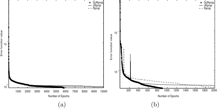
[image:11.612.103.476.22.211.2](a) (b)
Fig. 1. GJRprop, JRprop and Rprop learning curves for (a) the cancer problem and (b) the diabetes problem
allk.
4.1 The Cancer1 problem
The breast cancer diagnosis problem is based on 9 inputs describing a tu-mour as benign or malignant. The data set consists of 350 patterns. We have used a feed-forward neural network with 9–4–2–2 nodes as suggested in the PROBEN1 benchmark collection and in [3]. The error goal in training was
E <0.02 to harmonize with the training errors obtained in [3,13]. The results
for this pattern classification problem are summarized in Table 1. The new algorithm performs significantly better than the other two methods. Table 2 presents the number of times each algorithm outperforms the other methods in terms of training speed and generalization within 150 independent runs. It yields that the new learning scheme is frequently faster and achieves better generalization than the other two members of the Rprop family. Figure 1(a)
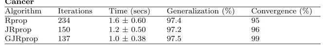
Table 1
Comparison of algorithms performance in the Cancer problem for the converged runs
Cancer
Algorithm Iterations Time (secs) Generalization (%) Convergence (%)
Rprop 234 1.6±0.60 97.4 95
JRprop 150 1.2±0.50 97.2 96
GJRprop 137 1.0±0.38 97.5 99
presents an example of convergence behavior starting from the same initial conditions: the Rprop converges to a local minimizer, whilst both JRprop and
GJRprop converge to a feasible solution (E ≤ 10−2) with GJRprop
[image:11.612.122.454.553.600.2]Table 2
Number of times, out of 150 runs, each algorithm performs better than the other methods in the Cancer problem with respect to training speed and generalization.
Cancer Times faster Times better algorithm Generalization
Algorithm Rprop JRprop GJRprop Rprop JRprop GJRprop
Rprop – 55 25 – 20 13
JRprop 93 – 57 42 – 36
GJRprop 125 102 – 53 50 –
4.2 The Diabetes1 problem
The aim of this real-world classification task is to decide when a Pima In-dian individual is diabetes positive or not. We have 8 inputs representing personal data and results from a medical examination. The data set consists of 384 patterns. The PROBEN1 collection proposes several architectures for this problem, including one with 8–2–2–2 nodes. We decided to use this ar-chitecture as it was also suggested by others [3,13]. The error goal in this case
was set at 0.14 to conform to the training error obtained in [3,13].
[image:12.612.146.427.419.464.2]Table 3 summarises the performance of the tested algorithms. The increased training speed does not affect the generalization performance of the new method. It is worth noting the standard deviation value of the GRprop is significantly less than the corresponding Rprop and JRprop values, which means GJRprop performance is closer to the average value. Table 4 gives an analytic view of the comparative results in the 150 trials.
Table 3
Comparison of algorithms performance in the Diabetes problem for the converged runs
Diabetes
Algorithm Iterations Time (secs) Generalization (%) Convergence (%)
Rprop 380 2.3±2.0 75.5 90
JRprop 310 1.9±1.5 75.4 93
[image:12.612.126.448.532.593.2]GJRprop 290 1.7±0.8 75.8 98
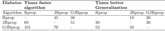
Table 4
Number of times, out of 150 runs, each algorithm performs better than the other methods in the Diabetes problem with respect to training speed and generalization.
Diabetes Times faster Times better algorithm Generalization
Algorithm Rprop JRprop GJRprop Rprop JRprop GJRprop
Rprop – 45 38 – 18 20
JRprop 68 – 51 30 – 20
GJRprop 101 70 – 52 50 –
Figure 1(b) illustrates a training instance where all the methods start under the same initial conditions: the Rprop converges to a local minimizer, whilst
4.3 The Escherichia coli problem
This problem concerns the classification of the Escherichia coli (E.coli) protein localization patterns into eight localisation sites. E.coli, being a prokaryotic gram-negative bacterium, is an important component of the biosphere. Three major and distinctive types of proteins are characterized in E.Coli: enzymes, transporters and regulators. The largest number of genes encodes enzymes (34%) (this should include all the cytoplasm proteins) followed by the genes for transport functions and the genes for regulatory proses (11.5%) [14].
In these experiments the neural networks were tested using 4–fold cross val-idation, as this approach has been used before in the literature for training probabilistic and nearest neighbor classifiers in this problem [12]. The best available architectures that was suggested is a 7–16–8 FNN [1]. Rprop–trained FNNs of this architecture achieved better generalization than the best results
reported in the literature [12], when the training error goal was E <0.02 [1].
[image:13.612.116.463.349.393.2]Results from 150 runs for three algorithms using the same architecture are given in Table 5. A detailed account of the algorithms’ performance is exhib-ited in Table 6. Figure 2(a) illustrates the behavior of the training algorithms
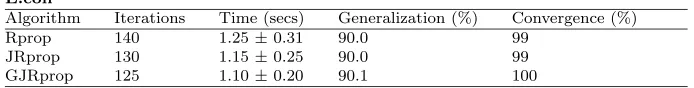
Table 5
Comparison of algorithms performance in the E.coli problem for the converged runs
E.coli
Algorithm Iterations Time (secs) Generalization (%) Convergence (%)
Rprop 140 1.25±0.31 90.0 99
JRprop 130 1.15±0.25 90.0 99
[image:13.612.119.459.436.497.2]GJRprop 125 1.10±0.20 90.1 100
Table 6
Number of times, out of 150 runs, each algorithm performs better than the other methods in the E.coli problem with respect to training speed and generalization.
E.coli Times faster Times better algorithm Generalization
Algorithm Rprop JRprop GJRprop Rprop JRprop GJRprop
Rprop – 62 61 – 55 49
JRprop 87 – 70 70 – 67
GJRprop 86 73 – 87 70 –
in a case where E ≤ 0.01. Convergence to a feasible solution is achieved by
GJRprop within 6000 iterations while the other schemes require more than 10000 iterations.
4.4 The Thyroid problem
In this problem, the aim is to find whether the patient’s thyroid has over
func-tion, normal funcfunc-tion, or under function. We have used the thyroid1 dataset
(3600 patterns), a network with 21–4–3 nodes, and the error goal was set at
1000 2000 3000 4000 5000 6000 7000 8000 9000 10000 10
-1
GJRprop JRprop Rprop
Error function value
Number of Epochs 10
-2
200 400 600 800 1000 1200 1400 1600 1800 2000 10-2
10-1
GJRprop JRprop Rprop
Number of Epochs
Error function value
[image:14.612.103.475.24.211.2](a) (b)
Fig. 2. GJRprop, JRprop and Rprop learning curves for (a) the E.coli problem and (b) the thyroid problem.
Comparative results are given in Table 7. GJRprop outperforms the other algorithms. Moreover, the value of the deviation of the new algorithm is sig-nificantly lower than the standard deviation of the other two methods (see Ta-ble 7). Finally it is worth mentioning that the GJRprop exhibits significantly improved convergence success compared to the other tested algorithms. This can be attributed to the ability of new globally convergent algorithm to follow descent directions.
[image:14.612.113.456.464.509.2]A detailed account of the algorithms’ performance is exhibited in Table 8. The new learning scheme is faster than Rprop and JRprop 86 and 84 times respectively. In terms of generalization success, GJRprop outperforms Rprop and JRprop 78 and 76 times respectively.
Table 7
Comparison of algorithms performance in the Thyroid problem for the converged runs
Thyroid
Algorithm Iterations Time (secs) Generalization (%) Convergence (%)
Rprop 710 23.90±12.5 98.12 87
JRprop 640 21.40±10.1 98.12 89
[image:14.612.132.447.545.605.2]GJRprop 620 19.90±7.5 98.23 95
Table 8
Number of times, out of 150 runs, each algorithm performs better than the other methods in the Thyroid problem with respect to training speed and generalization.
Thyroid Times faster Times better algorithm Generalization
Algorithm Rprop JRprop GJRprop Rprop JRprop GRprop
Rprop – 71 64 – 66 57
JRprop 79 – 66 69 – 60
GJRprop 86 84 – 78 76 –
for the Rprop, and the other around point 200 for the JRprop. The GJR-prop decreases monotonically the error function as it always follows a descent direction.
4.5 Boolean function approximation problems
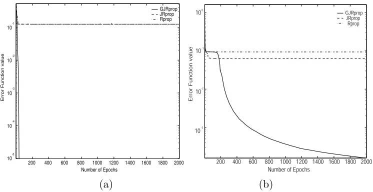
Another set of experiments has been conducted to empirically evaluate the performance of the globally convergent method in a well–studied class of boolean function approximation problems that exhibit strong local minima and stationary points [6,9]. These problems include the XOR problem (whose local minina and saddle points have been analyzed in detail) and the various
parity–N problems, which are considered as classic benchmarks [16,21,33].
The adopted architectures were 2–2–1 for the XOR, 3–3–1 for the parity–3, 4–4–1 for the parity–4, 5–5–1 for the partiy–5.
For the XOR problem the error target was set to E 6 10−5 within 2000
iterations and for the parity-5 problem was set toE 610−6, while for the other
remaining boolean function approximation problems the acceptable solution
was set atE 65×10−5. All these target values are considered low enough to
guarantee convergence to a “global” solution.
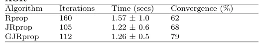
4.5.1 XOR problem
[image:15.612.157.417.546.590.2]Table 9 shows the performance of each algorithm. GJRprop exhibits better convergence success than other methods: GJRprop achieved 79% average con-vergence success, while Rprop and JRprop achieved on average 62% and 68%. The GJRprop outperforms significantly over the Rprop in terms of conver-gence speed and relatively similar speed with the JRprop.
Table 9
Comparison of algorithms performance in the XOR problem for the converged runs
XOR
Algorithm Iterations Time (secs) Convergence (%)
Rprop 160 1.57±1.0 62
JRprop 105 1.22±0.6 68
GJRprop 112 1.26±0.5 79
200 400 600 800 1000 1200 1400 1600 1800 2000 10
-5
10
-4
10
-3
10
-2
10
-1
Number of Epochs
Error Function value
GJRprop JRprop Rprop
200 400 600 800 1000 1200 1400 1600 1800 2000
10-3 10 -2 10 -1
100
Number of Epochs
Error Function value
GJRprop Rprop JRprop
[image:16.612.103.476.19.211.2](a) (b)
Fig. 3. Learning error curves for (a) the XOR problem and (b) the parity–3
4.5.2 Parity–3 problem
[image:16.612.164.409.464.510.2]Table 10 presents comparative results in terms of training speed (in secs) and convergence success for the 150 runs. It presents the average training time and the corresponding standard deviation for each algorithm calculated over the converged runs. GJRprop shows an increase in the percentage of convergence success. The globally convergent scheme manages to escape from some local minima and finds acceptable solutions with higher possibility than the other two tested methods do. Finally Figure 3(b) shows a case where Rprop and JRprop converge to local minima while GJRprop reaches a minimiser with lower function value for the parity–3 problem.
Table 10
Comparison of algorithms performance in the parity–3 problem for the converged runs
Parity–3
Algorithm Iterations Time (secs) Convergence (%)
Rprop 885 3.8±1.9 79
JRprop 850 3.5±1.6 77
GJRprop 840 3.3±1.3 88
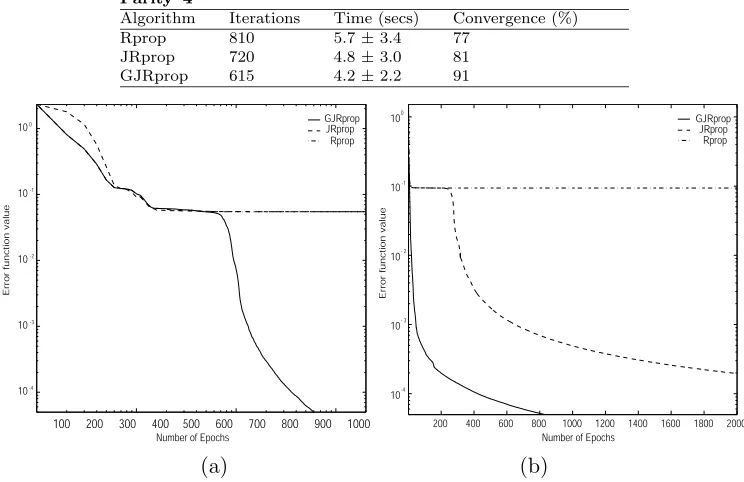
4.5.3 Parity–4 problem
Table 11
Comparison of algorithms performance in the parity–4 problem for the converged runs
Parity–4
Algorithm Iterations Time (secs) Convergence (%)
Rprop 810 5.7±3.4 77
JRprop 720 4.8±3.0 81
GJRprop 615 4.2±2.2 91
10-4 10 -3 10 -2 10 -1 100
Number of Epochs
Error function value
GJRprop Rprop JRprop
100 200 300 400 500 600 700 800 900 1000 200 400 600 800 1000 1200 1400 1600 1800 2000
10-4 10- 3 10 - 2 10 -1 100
Number of Epochs
Error function value
GJRprop Rprop JRprop
(a) (b)
Fig. 4. Typical learning error curves for (a) the parity–4 problem and (b) the par-ity–5 problem.
4.5.4 Parity–5 problem
[image:17.612.160.417.497.542.2]Comparative results for the parity–5 problem are presented in Table 12. The JRprop algorithm achieves the best training speed, while GJRprop exhibits comparable performance. Both of them outperform the Rprop algorithm. Fur-thermore the GJRprop is more stable and shows an important convergence improvement over the other tested methods. Figure 4(b) illustrates a case where GJRprop converges to an acceptable minimiser while the other meth-ods converge to local minima with higher function values.
Table 12
Comparison of algorithms performance in the parity–5 problem for the converged runs
Parity–5
Algorithm Iterations Time (secs) Convergence (%)
Rprop 950 6.7±3.6 61
JRprop 760 4.1±2.0 64
GJRprop 795 4.5±2.1 82
5 Conclusions
better training speed than Rprop and JRprop in six out of the eight bench-marks, and demonstrated stability in locating minimisers with high percentage of success in all cases. The comparative study reported in the paper also shows that GJRprop exhibits more consistent behavior than the other algorithms. Nevertheless, we acknowledge that this is a small scale study. Further research into the performance of the method is needed to fully explore its advantages and identify possible limitations in pattern recognition problems.
References
[1] Anastasiadis A.D., Magoulas G.D., and Liu X., Classification of protein localisation patterns via supervised neural network learning, In: Proceedings of
theFifth Symposium on Intelligent Data Analysis (IDA-03), Berlin, Germany,
August 2003, Lecture Notes in Computer Science, vol. 2810, Springer-Verlag, 430–439.
[2] Anastasiadis A.D., Magoulas G.D., Vrahatis M.N., An efficient improvement of the Rprop algorithm, In: Proceedings of the 1st International Workshop on
Artificial Neural Networks in Pattern Recognition (IAPR 2003), University of
Florence, Italy, pp.197–201, 2003.
[3] Anastasiadis A.D., Magoulas G.D., Vrahatis M.N., Sign-based learning schemes for pattern classification,Pattern Recognition Letters, forthcoming.
[4] Battiti R., First-and second-order methods for learning: Between steepest descent and Newton’s method,Neural Computation, 4, 141–166, 1992.
[5] Bishop C.M.,Neural Networks for Pattern Recognition, Oxford, 1995.
[6] Blum E.K., Approximation of Boolean functions by sigmoidal networks: Part I: XOR and other two variable functions, Neural Computation, 1, 532–540, 1989. [7] Burton R. M. and Mpitsos G. J., Event dependent control of noise enhances
learning in neural networks,Neural Networks, 5, 627-637, 1992.
[8] Dennis J. E. and Schnabel R. B., Numerical Methods for Unconstrained
Optimization and Nonlinear Equations, SIAM, Philadelphia, 1996.
[9] Gori M. and Tesi A., On the problem of local minima in backpropagation,IEEE
Trans. Pattern Analysis and Machine Intelligence, 14, 76–85, 1992.
[10] Haykin S.,Neural Networks: A Comprehensive Foundation, Macmillan College Publishing Company, 1994.
[11] Hertz J., Krogh A. and Palmer. R, Introduction to the Theory of Neural
Computation, Addison Wesley, 1991.
[12] Horton P. and Nakai K., Better prediction of protein cellular localization sites with theknearest neighbors classifier, In: Proceedings of theIntelligent Systems
[13] Igel C. and Husken M., Empirical evaluation of the improved Rprop learning algorithms,Neurocomputing, 50, 105–123, 2003.
[14] Liang P., Labedan B. and Riley M., Physiological genomics of Escherichia coli protein families,Physiological Genomics, 9, 1, 15–26, 2002.
[15] Magoulas G.D., Vrahatis M.N., Grapsa T.N. and Androulakis G.S., Neural network supervised training based on a dimension reducing method, In: S.W. Ellacot, J.C. Mason, and I.J. Anderson (eds.), Mathematics of Neural
Networks: Models, Algorithms and Applications, Kluwer, pp.245–249, 1997.
[16] Magoulas G.D., Vrahatis M.N. and Androulakis G.S., Effective back-propagation training with variable stepsize,Neural Networks, 10, 69–82, 1997.
[17] Magoulas G.D., Vrahatis M.N. and Androulakis G.S., Improving the convergence of the backpropagation algorithm using learning rate adaptation methods,Neural Computation, 11, 1769–1796, 1999.
[18] M¨oller M.F., A scaled conjugate gradient algorithm for fast supervised learning,
Neural Networks, 6, 525–533, 1993.
[19] Murphy P.M. and Aha D.W., UCI Repository of machine learning databases, Irvine, CA: University of California, Department of Information and Computer Science, 1994. http://www.ics.uci.edu/ mlearn/MLRepository.html.
[20] Nocedal J., Theory of algorithms for unconstrained optimization, Acta
Numerica, pp.199–242, 1992.
[21] Plagianakos V.P., Magoulas G.D. and Vrahatis M.N., Learning in multilayer perceptrons using global optimization strategies, Nonlinear Analysis: Theory,
Methods and Applications, 47, 3431–3436, 2001.
[22] Plagianakos V.P., Magoulas G.D. and Vrahatis M.N., Supervised training using global search methods, N. Hadjisavvas and P. Pardalos (eds.), Advances in Convex Analysis and Global Optimization, vol. 54, Noncovex Optimization and
its Applications, Kluwer Academic Publishers, Dordrecht, The Netherlands,
pp.421-432, 2001.
[23] Prechelt, L., PROBEN1-A set of benchmarks and benchmarking rules for neural network training algorithms, T.R. 21/94, Fakult¨at f¨ur Informatik, Universit¨at, Karlsruhe, 1994.
[24] Riedmiller M. and Braun H., A direct adaptive method for faster backpropagation learning: The Rprop algorithm, In: Proceedings of the
International Conference on Neural Networks, San Francisco, CA, pp.586-591,
1993.
[25] Riedmiller M., Rprop - Description and Implementation Details Technical Report, University of Karlsruhe, January 1994.
Computer Standards and Interfaces, Special Issue on Neural Networks, 16, 265-278, 1994.
[27] Rumelhart D.E. and McClellend J.L., Parallel Distributed Processing:
Explorations in the Microstructure of Cognition, Cambridge, MIT Press,
pp.318-362, 1986.
[28] Scales L. E., Introduction to Non-linear Optimization, MacMillan Publishers, LTD, pp.34–35, 1985.
[29] Sikorski, K.,Optimal Solution of Nonlinear Equations, Oxford University Press, New York, 2001.
[30] Treadgold N.K. and Gedeon T.D., Simulated annealing and weight decay in adaptive learning: The SARPROP algorithm, IEEE Trans. Neural Networks, 9, 4, 662-668, 1998.
[31] Vrahatis M.N., Solving systems of nonlinear equations using the nonzero value of the topological degree,ACM Trans. Math. Software, 14, 312–329, 1988; ibid: 14, 330–336, 1988.
[32] Vrahatis M.N., Magoulas G.D. and Plagianakos V.P., From linear to nonlinear iterative methods,Appl. Numer. Math., 45, 1, 59–77, 2003.
[33] Van der Smagt P.P., Minimization Methods for training feedforward neural networks.Neural Networks, 7, 1–11, 1994.