www.hydrol-earth-syst-sci.net/14/1567/2010/ doi:10.5194/hess-14-1567-2010
© Author(s) 2010. CC Attribution 3.0 License.
Hydrology and
Earth System
Sciences
A method for parameterising roughness and topographic sub-grid
scale effects in hydraulic modelling from LiDAR data
A. Casas1,4, S. N. Lane2, D. Yu3, and G. Benito1
1Institute of Natural Resources, Consejo Superior de Investigaciones Cient´ıficas, 28006 Madrid, Spain
2Institute Hazard, Risk and Resilience and Department of Geography, Durham University, Durham, DH1 3LE, UK 3Department of Geography, Loughborough University, Loughborough, LE11 3TU, UK
4Department of Land, Air, and Water Resources, University of California, Davis, CA 95616, USA Received: 16 March 2010 – Published in Hydrol. Earth Syst. Sci. Discuss.: 12 April 2010 Revised: 28 July 2010 – Accepted: 3 August 2010 – Published: 17 August 2010
Abstract. High resolution airborne laser data provide new
ways to explore the role of topographic complexity in hy-draulic modelling parameterisation, taking into account the scale-dependency between roughness and topography. In this paper, a complex topography from LiDAR is processed using a spatially and temporally distributed method at a fine reso-lution. The surface topographic parameterisation considers the sub-grid LiDAR data points above and below a reference DEM, hereafter named as topographic content. A method for roughness parameterisation is developed based on the topo-graphic content included in the topotopo-graphic DEM. Five sub-scale parameterisation schemes are generated (topographic contents at 0,±5, ±10,±25 and±50 cm) and roughness values are calculated using an equation based on the mix-ing layer theory (Katul et al., 2002), resultmix-ing in a co-varied relationship between roughness height and topographic con-tent. Variations in simulated flow across spatial subscales show that the sub grid-scale behaviour of the 2-D model is not well-reflected in the topographic content of the DEM and that subscale parameterisation must be modelled through a spatially distributed roughness parameterisation. Variations in flow predictions are related to variations in the roughness parameter. Flow depth-derived results do not change sys-tematically with variation in roughness height or topographic content but they respond to their interaction. Finally, sub-scale parameterisation modifies primarily the spatial struc-ture (level of organisation) of simulated 2-D flow linearly with the additional complexity of subscale parameterisation.
Correspondence to: A. Casas ([email protected])
1 Introduction
as diffusive effects in flow due to turbulence in a 2-D ap-proach). Therefore, the roughness parameter turns out to be an effective parameter commonly obtained through a calibra-tion procedure (e.g. Lane and Ferguson, 2005; Hunter et al., 2007). This situation complicates the scale-dependent rela-tionship between roughness and topography.
However, the growth of hydraulic modelling applications has emphasized the importance and necessity of innova-tion in terms of processes representainnova-tion, mainly in relainnova-tion to boundary roughness parameterisation (Lane et al., 2004; Nicholas, 2005; Horritt, 2005; Carney et al., 2006) and topo-graphic parameterisation methodologies (Bates et al., 2003; Leclerc, 2005, Casas et al., 2010). This is particularly the case in the light of new possibilities for technical advances in remote sensing, topographic data collection and spatial analysis techniques. At the same time, the recent increasing availability of high resolution LiDAR data for representing complex surfaces in detail (Marks and Bates, 2000; Bates et al., 2003; Suarez et al., 2005; Andersen et al., 2006; Man-dlburger and Briese, 2007; Liu, 2008; Cook and Merwade, 2009) and extracting vegetation density and height (Popescu and Zhao, 2008; Antonarakis et al., 2007, 2008) are promot-ing the development of new resistance formulations to link this highly detailed information with the spatially-averaged flow dynamics simulated by the model (Katul et al., 2002; Poggi et al., 2008, 2009). LiDAR measurement principles are well established (Ackermann, 1999; Wehr and Lohr, 1999) but the processing of raw data and the accuracy of re-sultant modelled data are not so evident (Gomes-Pereira and Wicherson, 1999; Hodgson and Bresnahan, 2004) although Marks and Bates (2000), Bates et al. (2003) and Mason et al. (2003) are important exceptions in relation to flood inun-dation modelling. Previous research on LiDAR applications to river hydraulics has addressed not only the influence of mesh resolution of processed laser data but that of the char-acteristic elements that modify the measurement scale, in-cluding the raw point density scheme and flying height in the measurement scale (Hirata, 2004), but also its particular im-pact upon flood modelling (Raber et al., 2003; Omer et al., 2003; Gueudet, 2004; Haile, 2005).
One of the main difficulties in the use of LiDAR data is the uncertainty introduced in the DEM, namely the errors due to the difficulty of filtering bare earth from the rest of measured data (e.g. Sithole and Vosselman, 2004). Low veg-etation is particularly difficult to differentiate from ground measurement (Asselman, 2002; Straatsma and Middelkoop, 2006). Filtering procedures are commonly used to classify bare earth from the rest of the points. Different filtering and classification procedures or criteria will lead to differ-ent modelled ground surfaces for a certain mesh resolution (Sithole and Vosselman, 2004). Points classified as terrain will determine the topographic content of the ground model, which in combination with mesh resolution determines the spatial scale of the elevation model. Thus, high resolution laser altimetry data cannot only be extremely useful for the
topographic parameterisation of a 2-D hydraulic model but also provide insight into the main set of problems related to scale in its spatial parameterisation (e.g. Hauer et al., 2009). LiDAR data can be used to control the topographic content introduced into a DEM generated for a fixed mesh resolu-tion. In this way, the assessment of spatial scale effects in hydraulic models can be performed by modifying exclusively the topographic content of the DEM (Casas et al., 2010).
This paper explores the role of topographic complex-ity considering a spatially and temporally distributed sub-scale parameterisation, where the roughness parameterisa-tion scheme varies with the amount of high resoluparameterisa-tion ge-ometric detail included in the topographic DEM. The main objectives are Eq. (1) to develop a subscale spatial param-eterisation methodology using LiDAR data that responds to the dependency of the model upon the topographic scale for a 2-D floodplain inundation model and Eq. (2) to assess its pa-rameterisations’ impacts upon the magnitude and the struc-ture of depth derived results. It must be noted that a precise characterisation of hydraulic roughness values is outside the scope of this study, and would require detailed field recording of hydraulic variables (discharge, depth, velocity, etc.) dur-ing a flood. A major contribution of this study is to account for the impact of topographic complexity below the scale of the model upon simulated flow taking advantage of the high resolution geometric detail provided by LiDAR map-ping sources. Our approach allows us: Eq. (1) to consider the topographic scale dependence in a distributed roughness parameterisation method; and Eq. (2) to separate the impact of the amount of topography included in the DEM at a certain modelling scale without introducing mesh resolution scaling impacts. Mesh resolution impacts upon subscale parameter-isation will be on the scope of further research in relation to the topographic impact across modelling scales.
2 Methodology
Our approach considers that the spatial scale of discretisation in the inundation model should act as a threshold for the rela-tive topographic and roughness parameterisation. Therefore, the roughness height (z0)can be determined as a function of the amount of topography (i.e. the topographic content,1z) contained within the discretised mesh, which conversely de-pend on the mesh resolution (m) of topographic and ness parameterisation. Hence, the topographic and rough-ness parameterisation should be connected through a three-way interaction between the mesh resolution, topographic content and the roughness parameterisation.
2.1 Digital terrain modelling and topographic content
34
818
819 820
Figure 1. Ortophoto with the location of the modelled reach (large rectangle) and the detailed rectangle 821
on the floodplain of the Ter River, near Sant Julià de Ramis (Girona, NE Spain). 822
823
Fig. 1. Ortophoto with the location of the modelled reach (large rectangle) and the detailed rectangle on the floodplain of the Ter River, near Sant Juli`a de Ramis (Girona, NE Spain).
±25cm
LiDAR point
DEM ±25c m
DEMref
(A)
Z
0 refZ±25c m
0
LiDAR points
DEMref
(B )
Zref 0
Z
0 refDref
Fig. 2. (A) Selection criteria for the incorporation of a LiDAR point within the topographic or roughness parameterisation procedure.
(B) Cell roughness calculation of averaged roughness height(D)
for a representation scale.
riparian vegetation, whereas most of the floodplain is occu-pied by field crops (cereals and alfalfa) and plots with poplar groves. For our purpose, a quadrilateral of 100 m by 50 m from the floodplain area was selected (Fig. 1). The selected area contains an array of vegetation types, including riparian vegetation (with different heights), poplar planted groves and crops.
0 10
20 30
40 50 0
20 40 60 80 10046
48 50 52
X (m) Y (m)
A
Z
(
m
)
0 10
20 30
40 50 0
20 40 60 80 10046
48 50 52
X (m) Y (m)
B
Z
(
m
[image:3.595.50.285.63.239.2])
Fig. 3. Generation of DEMs with additional topographic
informa-tion. (A) Reference DEM, (DEMref); (B) DEM with additional
to-pographic content of±25 cm (DEM±25cm). The origin of the plot
corresponds to the corner of the detailed rectangle in Fig. 1, which is downstream and closer to the river bank.
[image:3.595.311.546.66.249.2] [image:3.595.49.286.305.551.2]Fig. 4. Onset of free shear turbulent flows in shallow streams, after Katul et al., 2002.
of LiDAR data will produce DEMs with greater height vari-ability which can be quantified using spatial statistics. In this study, the semivariance and Geary’s C spatial autocorrelation index (Cliff and Ord, 1973) are used.
2.2 Roughness parameterisation
LiDAR-derived roughness height (z0)values for each cell of the modelled surface permits an objective estimation of the flow resistance for each cell of the 2-D floodplain inundation model. This study uses a new mixing layer theory for flow re-sistance in shallow streams developed by Katul et al. (2002). This approach predicts flow resistance from surface rough-ness measures and water depth using a mixing layer analogy rather than the standard rough-wall boundary layer theory. The mixing layer theory with its inflectional profile yields mean flow velocities at high relative roughness, providing analytical linkage between depth, roughness, and velocity for h/z0<7 wherehis water depth andz0roughness height.
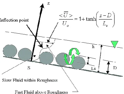
The approach makes use of the turbulent flow structure within and above rigid vegetation canopies. The structure of the flow near extensive and porous roughness elements resembles a mixing layer with an inflection near the mean height of the roughness element(D), Fig. 4, (Raupach et al., 1996, cited by Katul et al., 2002) whereas rough-wall bound-aries do not possess an inflection point (Katul et al., 2002).
The theory acknowledges that the mean velocity within the roughness element is small, while above the roughness element the mean velocity is large. Inflectional profiles are reproduced using a mean velocity equation given by:
U U0
=1+tanh
z−D
Ls
(1) whereD is the mean height of the roughness elements;Ls
is a characteristic energetic eddy size (i.e., mixing length)
produced atz=DandU0is the mean reference velocity at
z=D. Following Katul et al. (2002), the depth-averaged velocity can result, forLs≈αD:
U u0
=1
h
Z h
0
1+tanh
z−D
αD
dz (2)
=1+αD
h ln
cosh1α− h αD
coshα1
By letting:u0=Cuu∗;ξ=Dh;
f (ξ,α)=1+α1 ξln
coshα1−1 αξ
coshα1
(3)
It can be expressed as:
U u∗
=Cuf (ξ,α) (4)
whereCuis a similarity constant andu∗is the friction
veloc-ity:
u∗= p
g,h,S (5)
whereSis the bed slope andhthe depth
The result in Eq. (4) is highly dependent on the definition ofD. Upon comparing Eqs. (4) and (5) and Manning’s equa-tion for a wide rectangular channel:
U=1 nh
2/3S1/2 (6)
a relation between the depth-averaged velocity and Man-ning’sncan be explicitly established:
n= h
1/6
√
gCuf (ξ,α)
(7) Values ofα=1 andCu=4.5 are recommended for a range
ofh/Dof between 0.2 and 7.
In this study, this equation incorporated into the 2-D flood model and a roughness value is obtained for each cell of the domain at every time step of the calculation. The mean height of the roughness element (D)is set to be the aver-aged value of the roughness height (z0)data located within a cell of the model mesh, wherez0is calculated as the dif-ference between the DEM and measured LiDAR point, (see Fig. 2b). Thus, the definition ofD, and thereforen, will de-pend upon the mesh resolution of the scheme. Therefore, the modelling scheme of the 2-D hydraulic model applied in this study requires a Digital Roughness Model (DRM) with D
[image:4.595.304.551.106.291.2]The methodology developed in this study to obtain a dis-tributed roughness parameterisation is based on roughness height information (z0)of non-terrain elements derived from LiDAR points recorded but not classified and thus not in-cluded in the terrain model generation as topographic content (1z), (see Fig. 2a). Therefore, using this scheme, roughness height (z0)estimation will be dependent on the topography used to generate the DEM and its mesh resolution. Where the DEM does not represent topography explicitly, the model accounts for it through the roughness height (z0).
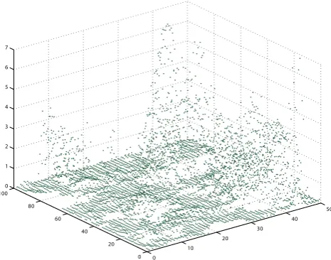
Roughness height calculation uses LiDAR altimetric data to which the elevation of the DEM is subtracted using a GIS routine (e.g. Cobby et al., 2001). The resultant roughness height (z0), which is the measured LiDAR data detrended from the terrain elevation (Fig. 5), was then interpolated to the corresponding mesh resolution(m)of the DEM into a DRM.
In this approach, it is assumed that the laser measures the range to any obstacle, which subsequently disturbs the flow pattern at a specific location. Thus, momentum roughness height (z0or the height at which velocity becomes zero) is considered to be the difference between the height at which the laser find the higher physical solid obstacle and the esti-mated terrain height at that location.
2.3 Hydraulic modelling
In this study, a hybrid 1-D/2-D hydraulic model (FloodMap) of flood inundation has been used. FloodMap (Yu and Lane, 2006a, b) is a coupled 1-D/2-D flood inundation model de-signed for fluvial flood inundation prediction in topographi-cally complex floodplains. It has a similar structure to that of JFLOW (Bradbrook et al., 2004). The model is the ba-sis of the sub-grid treatment approach developed by Yu and Lane (2006b) and has been tested and verified with a range of boundary conditions and in a number of environments (Yu, 2005; Tayefi et al., 2007; Lane et al., 2007; Lane et al., 2008). Yu and Lane (2006a) have reviewed the basis of the model, and so only the major model structure is outlined here. The coupled model assumes that the floodplain is pro-tected by an embankment that essentially acts as a contin-uous, broad-crested weir through which flow exchange oc-curs between the channel and floodplain. A tightly-coupled approach solves the one-dimensional river flow and two-dimensional floodplain flows simultaneously in a raster envi-ronment. The one-dimensional in-channel model solves the full Saint-Venant equations for unsteady open-channel flow using the Preissmann scheme based upon the fixed bed model of Abbott and Basco (1989).
The floodplain flow is simulated with a 2-D diffusion-based approach diffusion-based on the discretisation of the Manning’s equation in a raster-based environment. The model is to-pography driven, and recognizes any change in topographic modelling scale in terms of small-scale flow characteristics
0 10
20 30
40 50
0 20 40 60 80 100
[image:5.595.311.544.63.246.2]0 1 2 3 4 5 6 7
Fig. 5. Detrended roughness heights for the 1m-resolution refer-ence DEM studied floodplain detail, (m). The origin of the plot corresponds to the corner of the detailed rectangle in Fig. 1, which is downstream and closer to the river bank.
and routing, water surface elevation and large-scale inunda-tion extent.
2.4 Model boundary conditions
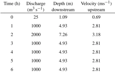
Three types of boundary conditions are required by the 1-D component of FloodMap, i.e. upstream and downstream flow hydrographs, river cross sectional geometry, and roughness parameter in each cross section. In terms of the flow bound-ary conditions, FloodMap can use a combination of either: (i) velocity downstream and stage upstream; or (ii) velocity upstream and stage downstream In addition, both options re-quire an estimation of water depth and velocity at each cross-section at the start of simulation, as initialisation data. This is summarized in Table 1. For this application, the second option is used.
There were no measured flow boundary conditions avail-able at the domain boundary of the study site to initialize the 1-D component of FloodMap. Instead, these were obtained from a one-dimensional hydraulic HEC-RAS model (Refer-ence of Army Corps of Engineers) implemented along a 2 km long river reach run for subcritical flow conditions (Casas et al., 2006). The associated water depth and velocity used here are shown in Table 2. For this reach, the flow boundary con-ditions required by FloodMap were calculated with an initial discharge of 25 m3s−1.
Table 1. Boundary condition requirements for the 1-D river model. (Option 2 is used in this study).
Upstream Downstream Upstream Downstream Depth at each Velocity at each
depth depth velocity velocity cross-section cross-section
Option 1 √ √ √
Option 2 √ √ √
Table 2. Inflow data.
Time (h) Discharge Depth (m) Velocity (ms−1)
(m3s−1) downstream upstream
0 25 1.09 0.69
1 1000 4.93 2.81
2 2000 7.26 3.18
3 1000 4.93 2.81
4 1000 4.93 2.81
5 1000 4.93 2.81
6 1000 4.93 2.81
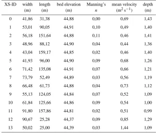
HEC-RAS modelling (Casas et al., 2006). In total thirteen cross sections were used in the study site. The associated boundary conditions required by the model are shown in Ta-ble 3. These boundary conditions are introduced in the model as ASCII files.
The model was run for the whole floodplain area for each DEM and the associated digital roughness model (DRM). Two-dimensional velocities and water surface ele-vation ASCII files were obtained for each simulation.
2.5 Characterisation of topography and modelled
flow fields
The level of organisation of the DEMs and simulated flow ac-cording to the topographic content or the roughness parame-terisation is quantified using spatial statistics. The semivari-ance statistic, which uses the squared differences between neighbouring pixel values, provide an idea of the vertical variability underlying each surface for a certain lag. A lag of 1 pixel has been selected, as it is the mesh resolution of DEMs, therefore each pixel is evaluated against its immedi-ate neighbour. Semivariance values quantify the increment in the variability of the DEM as the vertical threshold1zof input data are increased (i.e. its topographic content)
Spatial autocorrelation, using Geary’s C index, has also been calculated for the scaled DEMs to quantify the homo-geneity in the spatial pattern of each DEM through the com-parison of neighbouring pixel values. Geary’s C uses the for-mula:
C(d)= (n−1)
n
P
i n
P
j
wij yi−yj
2
2W
n
P
i
zi2
(8)
Wherewijis the weight at distanced,z’s are deviations from
the mean for variabley, andW is the sum of all the weights wherei6=j. The value ranges from 0.0 to 3.0, with 0.0 for a strong positive spatial autocorrelation and + 1 for no corre-lation. Values from 1.0 to 3.0 indicate negative correcorre-lation.
3 Results
Firstly, the distributed roughness parameterisation method-ology developed is evaluated and the topographic content of DEMs is quantified. Secondly, scaling effects upon hydraulic model results due to roughness parameterisation and varia-tions in the topographic content of the DEM are assessed. Thereafter, the topographic content impact is isolated and the level of organisation of depth results is quantified through the Geary’s C spatial autocorrelation index Eq. (8). Finally, the full area is considered and model results are evaluated.
Descriptive statistics and semivariance values for each DEM are summarized in Table 4. Semivariance values in-crease as the models comprise more topographic content for a fixed mesh resolution. In addition, the spatial autocorre-lation Geary’s C index Eq. (8) has been calculated to com-pare the homogeneity between these DEMs as topographic content is introduced. Table 4 shows that Geary’s C spatial autocorrelation index increases as larger topographic content is introduced.
Table 5 summarises the statistics of roughness parameter-isation (n, from Eqs. 2 and 3) for the 2nd and 4th h of the simulation according to each scaled scheme for the detailed studied floodplain area. The Table shows that the Manning’s
[image:6.595.69.266.205.332.2]Table 3. Model geometry and boundary conditions estimated for an initial discharge of 25 m3s−1.
XS-ID width length bed elevation Manning’s mean velocity depth
(m) (m) (m) n (m2s−1) (m)
0 41,86 31,38 44,88 0,00 0,69 1,43
1 53,01 90,05 44,91 0,10 0,49 1,40
2 56,18 151,64 44,88 0,11 0,46 1,41
3 48,96 88,12 44,90 0,04 0,44 1,36
4 43,04 159,17 44,85 0,02 0,46 1,40
5 41,93 96,00 44,90 0,09 0,68 1,26
6 71,42 135,08 44,91 0,07 0,66 1,21
7 73,79 52,49 44,89 0,03 0,56 1,19
8 66,48 61,73 44,88 0,04 0,73 1,12
9 55,13 124,05 44,84 0,07 0,52 1,09
10 61,84 125,66 44,86 0,09 0,54 1,00
11 91,80 157,86 44,81 0,02 0,51 0,99
12 90,67 25,28 44,37 0,09 0,85 1,29
[image:7.595.125.470.408.527.2]13 50,02 25,00 44,39 0,03 1,44 1,09
Table 4. Descriptive statistics for each scaled DEM.
Statistics DEMref DEM±5cm DEM±10cm DEM±25cm DEM±50cm
Mean (m) 53.386 53.386 53.387 53.392 53.399
Minimum (m) 44.445 44.445 44.445 44.393 44.393
Maximum (m) 75.609 75.609 75.609 75.609 75.609
Std. Dev. (m) 2.896 2.896 2.896 2.897 2.896
Semivariance (m) 0.000159 0.000159 0.00016 0.000168 0.000183
Geary’s C 0.00376 0.00377 0.00385 0.00446 0.00562
Figure 6 shows, for the detailed studied floodplain area (Fig. 1), the input data (roughness heights (Fig. 6a) and model derived depths (Fig. 6b) required to calculate the dis-tributed roughness parametern(Fig. 6c). Roughness heights and roughness parameter are correlated (Fig. 6) where Man-ning’snvalues vary from 0.036 to 0.25 for a range of 0.02– 5.6 m of roughness heights,. This is confirmed in Table 5 where correlation coefficient(r)of Manning’snparameter in relation to roughness height (z0)and topographic elevation (DEM) is calculated as a measure of the agreement between model components.
Table 5. Statistics of roughness parameter(n)due to variations in the topographic content of the DEM (1z) and the roughness height (z0)
of the DRM for a detailed area (Fig. 1).
nref(2 h) n5cm(2 h) n10cm(2 h) n25cm(2 h) n50cm(2 h)
mean 0.072 0.075 0.072 0.074 0.072
max 0.260 0.259 0.260 0.259 0.260
min 0.034 0.030 0.035 0.033 0.034
std. dev. 0.050 0.054 0.049 0.052 0.050
r(z0) 0.882 0.849 0.884 0.867 0.875
r(DEM) 0.459 0.490 0.455 0.474 0.460
nref(4 h) n5cm(4 h) n10cm(4 h) n25cm(4 h) n50cm(4 h)
mean 0.067 0.068 0.067 0.068 0.067
max 0.260 0.260 0.259 0.260 0.260
min 0.038 0.037 0.038 0.038 0.038
std. dev. 0.041 0.043 0.041 0.042 0.041
r(z0) 0.930 0.923 0.931 0.927 0.929
r(DEM) 0.389 0.402 0.387 0.395 0.387
39
844 845
846
Figure 6. (a) Input map of roughness heights for a 1 m resolution of detailed area. (b) Model estimated 847
depths at the second hour. (c) Derived hydraulic roughness map calculated by the model at the second 848
hour. 849 850
Value
High : 7.34 m
Low : 0.28 m
Value
High : 5.57 m
Low : 0.02 m
Value
High : 0.25
Low : 0.04
A B C
Fig. 6. (A) Input map of roughness heights for a 1 mm resolution of detailed area. (B) Model estimated depths at the second hour. (C) Derived hydraulic roughness map calculated by the model at the second hour.
is not systematic with the linear increment of the topo-graphic subscale complexity that results from variation in the topographic content of the DEM and roughness height. Therefore, the roughness parameterisation model is sensi-tive to interactions between distributed roughness height and topographic content. The distributed scale-dependent methodology comprises the interaction between topography and roughness. Figure 7b shows, the comparison (RMSD) between flow depth results using models with additional
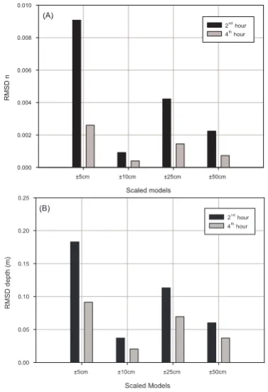
Fig. 7. RMSD values for (A) the roughness parameter and (B) depth
derived results when different subscale scheme results (±5,±10,
±25,±50 cm) are compared with those obtained using a reference
[image:8.595.50.287.359.533.2] [image:8.595.333.522.361.637.2]A. Casas et al.: Roughness and topographic sub-grid scale effects in hydraulic modelling 1575
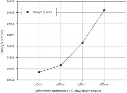
Fig. 8. Geary’s autocorrelation spatial index the percentages of dif-ferences normalised of flow depth results using each scheme com-pared with those obtained using a reference one (Ref).
subscale complexity (±5,±10,±2 5and±50) with those obtained using a reference one without additional complex-ity (Ref). The figure shows that the impact is not systematic with the linear increment of the topographic subscale com-plexity. However, from the comparison of Fig. 7a and b, it can be noted that variations (RMSD) in flow depth results are systematic with variations (RMSD) in roughness parameter-isation.
The percentages of the normalised differences of the depth derived results using each scaled scheme in relation to the reference one (DEMref)and the Geary’s C spatial autocor-relation index have been calculated. Figure 8 shows how, as the spatial subscale scheme becomes more complex and from
±5 cm toward ±50 cm, the autocorrelation index is closer to 1, which implies lower organisation in the flow. Figure 9 corroborates visually this impact on the structure of the flow, where it is shown how for the subscale scheme (i.e. account-ing for more topographic variation at±50 cm) the flow is less organised (Fig. 9a).
In order to isolate the impact of the topographic content of the DEM, the model has been simulated for a constant value of roughness height of 0.02 m, which results in a mean roughness value for the rectangle area of 0.043±0.004 and 0.044±0.003 at the 2nd and 4th h of the simulation. This is calculated for each one of the five simulations with dif-ferent topographic content in the DEM. Variations (RMSD) in depth results due to this constant roughness parameterisa-tion are of 0, 0.01, 0.02 and 0.03 when each model (±5 cm,
±10 cm,±25 cm,±50 cm) is compared with the reference one. From these results, it can be stated that for a constant value of roughness height: (i) the roughness parameterisa-tion is not globally sensitive to variaparameterisa-tions in the topographic content of the DEM; and (ii) the RMSD of depth varies pos-itively, increasing with the increment of topographic content in the 1 m-DEM, though in a very reduce quantity. There-fore, flow variability of the 2-D hydraulic model for a given
42
863
864
Figure 9. Percentages of differences normalised of flow depth results using each subscale scheme, 865
namely ± 50cm (a), ± 25 cm (b), ± 10 cm (c), ± 5 cm (d) compared with those obtained using a 866
reference one (Ref). 867
868
(A) %dn±50cm (B) %dn±25cm (C) %dn±10cm (D) %dn±5cm
Value
High : 28.75
Low : ï89.10
Fig. 9. Percentages of differences normalised of flow depth
re-sults using each subscale scheme, namely±50 cm (A),±25 cm
(B),±10 cm (C),±5 cm (D) compared with those obtained using
a reference one (Ref).
mesh resolution (close to measured topographic resolution) relies upon the interactions between topographic variability (1z) and roughness parameterisation(n), the former with a stronger and non-linear impact.
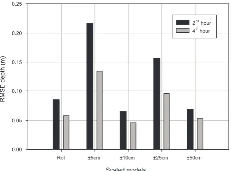
Depth derived results obtained using a distributed rough-ness parameterisation have been compared (RMSD) with those model results obtained using the same roughness pa-rameterisation methodology but a constant roughness height (Fig. 10). Figure 10 shows that the impact (RMSD) of us-ing a constant or a distributed roughness parameterisation ac-cording to surface characteristics is larger than the impact of using one topographic model or another (Fig. 7b).
Finally, Table 6 summarises the roughness parameterisa-tion impacts upon depth and inundaparameterisa-tion extent results at the 2nd and 4th h of the simulation for the full floodplain area. Variations (RMSD and percentage of differences normalised) are compared with the reference simulation results, show-ing a higher scalshow-ing effects on the inundation extent than on depth modelling results
4 Discussion
In river analysis, topography data and hydraulic roughness are major inputs to define terrain geometry.
Although scale dependency of roughness parameterisation upon represented topography is conceptually accepted, there are fewer studies quantifying the degree of this dependency (e.g. Lane, 2005; Horritt, 2005). Here we present a method to downscale topography using LiDAR geometric information and to include roughness content with physically meaningful criteria.
[image:9.595.309.549.66.168.2]Fig. 10. RMSD values for depth derived results obtained with a distributed roughness parameterisation are compared with those ob-tained using a constant roughness height, for the 2nd and 4th h of the simulation.
the topographic model. The theory provides a neat analyt-ical link between roughness and water depth and velocity, though it must be noted that ignores reduced resistance due to bending of vegetation and alignment of foliage with flow at higher velocities (Kouwen and Li, 1980; Kouwen and Fathi-Moghadam, 2000). The method encapsulates the three-way interaction between the discretised mesh resolution, the topo-graphic content of the DEM and the roughness parameterisa-tion and shows how subscale roughness parameterisaparameterisa-tion in-fluence flood depth and inundation extent. Furthermore, this approach has provided a suitable method not only to quan-tify the roughness properties of the surface but also to test the sensitivity of the hydraulic parameters to a distributed rough-ness parameterisation approach versus a constant roughrough-ness value.
Downscaled analysis shows that variations in flow depth are systematic with variations in the subscale parameteri-sation and not in relation to the topographic content of the DEM. In fact, when a constant value of roughness height of 0.02 m (bare ground conditions) is applied, the sub-scale behaviour of the simplified 2-D raster based model is not well-reflected through the topographic content of the DEM. Therefore, subscale flow variations must be mod-elled through a spatially distributed roughness parameterisa-tion that can retain small-scale topographic variaparameterisa-tions within coarse scale models. This implies the convenience of select-ing an adequate model scale accordselect-ing to the computselect-ing and application demands of the hydraulic model given the low level impact of topographic variability within a certain mesh cell. It also emphasises the importance of including geomet-ric shape details in the hydraulic computation mesh in accor-dance with some previous studies (Mandlburger et al., 2009; Schubert et al., 2008). This result may also play down the role of the filtering method used to classify ground points and
Table 6. Scaling effect upon depth derived results (RMSD) and in-undation extent (differences normalised %) due to subscale param-eterisation for the full area at the 2nd and 4th h of the simulation,
compared with the reference model (DEMref1m)simulation results.
Scaled RMSD Depth [m] Inundation extent [dn\%]
Models 2nd h 4th h 2nd h 4th h
DEMref 0.0000 0.0000 0.0000 0.0000
DEM5cm 0.0701 0.0490 0.4460 0.0060
DEM10cm 0.0548 0.0433 −0.4700 0.3450
DEM25cm 0.0592 0.0433 0.0300 0.1940
DEM50cm 0.0634 0.0525 0.1360 0.0240
its known problems in distinguishing between terrain points and low vegetation (Doneus and Briese, 2006) using raster-based hydraulic models in rural areas, where only features at the model scale modify depth-derived results.
Our results show that parameterisation process not only influences depth and flood extent but also the structure of the depth derived results. Figure 9 depicts the importance of the topographic variability bellow the modelling scale upon the level of organisation of spatially distributed hydraulic re-sults. The main implication of this sub-scale variation upon flow complexity results, according to the complexity of the spatial subscale scheme, is that a distributed subscale param-eterisation impacts not only on the range of depth results, as the global RMSD values show, but also modify the char-acteristic scale of flow results. This variation on the level of organisation of modelled flow, as controlled by the down scaled topography at a given mesh resolution, may be impor-tant for some ecological applications, such as habitat avail-ability where the river geometry at different scales plays a de-cisive role (Hauer et al., 2008; Lane and Carbonneau, 2007). In addition, this analysis emphasises the need for more com-prehensive consideration of the impact of scale on dominant processes and parameter sensitivity (Bates et al., 2005).
[image:10.595.313.543.125.239.2]The results obtained in this work agree with previous work in which distributed roughness can have a non-linear im-pact on flow results (Horritt et al., 2006; Nicholas, 2005). Importantly, this work identifies a change in the spatial struc-ture of the flow according to the organisation of downscaled topography, improving the insight of the performance of the model in relation to the structure and level of organisation of derived results at the modelling scale. This is important not only to design the modelling scheme but in the validation process. Data chosen to validate a model should reflect what the model must predict (Lane et al., 2005), then the required detailed variability in model results or the spatial structure of available validation data can drive the scale choice of the topographic and roughness parameterisation and should be taken into account in the modelling process. Further develop-ment of this method should address validation with spatially distributed field data.
5 Conclusions
The spatial scale dependency of a 2-D raster-based diffusion-wave model upon topographic subscale representation and parameterisation using a distributed spatially and temporally variable roughness parameterisation was assessed. This anal-ysis was based on laser altimetry data (LiDAR) and spatial analysis methods. A methodology to generate a roughness parameterisation model within the hydraulic model has been developed using down-scaled topographic data. The method explicitly recognises the three-way interaction between the discretised mesh resolution and the topographic content in the DEM with the roughness parameterisation. Subscale pa-rameterisation has been shown to impact depth and inun-dation extent derived results. The impact of using a con-stant or a distributed roughness parameterisation according to surface characteristics is larger than the impact of using one topographic model or another. Variations in flow results were found to be systematically related to variations in the roughness parameter. The subscale behaviour of the 2-D hy-draulic model is not well-reflected through the topographic content of the DEM and subscale parameterisation must be modelled through a spatially distributed roughness parame-terisation. Subscale parameterisation modifies primarily the spatial structure (level of organisation) of simulated 2-D flow linearly with the complexity of subscale parameterisation. This work suggests that a spatially distributed roughness pa-rameterisation provides a control in its impact upon the spa-tial distribution of model-derived results, therefore, upon its scale. Furthermore, our approach can be applied to cross-verify the accuracy of spatially distributed field data (e.g. water levels, flow velocity, depth) as well as to design a strat-egy on field measurements requirements for model valida-tion. There is a clear need to merge these results with varia-tions in the mesh resolution as it may also influence hydraulic modelling results.
Acknowledgements. The authors would like to thank the ICC (Institut Cartographic de Catalunya), especially Antonio Ruiz, for the provision of the LiDAR data used in this study. Finally, we are grateful to the reviewers, D. C. Mason and G. J.-P. Schumann, whose comments helped to improve the original manuscript.
Edited by: N. Verhoest
References
Abbott, M. B. and Basco, D. R.: Computational fluid dynamics, Longman Scientific and Technical with John Wiley & Sons, New York, 1989.
Ackermann, F.: Airborne laser scanning – present status and future expectations, ISPRS J. Photogramm., 54, 64–67, 1999.
Anderson, E. S., Thompson, J. A., Crouse, D. A., and Austin, R. E.: Horizontal resolution and data density effects on re-motely sensed LIDAR-based DEM, Geoderma, 132(3–4), 406– 415, doi:10.1016/j.geoderma.2005.06.004, 2006.
Antonarakis, A. S., Richards, K. S., and Brasington, J.: Object-based land cover classification using airborne LiDAR, Remote Sens. Environ., 112, 2988–2998, 2008.
Antonarakis, A. S., Richards, K. S., Brasington, J., Bithell, M., and Muller, E.: Retrieval of vegetative fluid resistance terms for rigid stems using airborne LiDAR, J. Geophys. Res., 113, G02S07, doi:10.1029/2007JG000543, 2008.
Asselman, N. E.: Laser altimetry and hydraulic roughness of veg-etation – further studies using ground truth, Technical report, Delft, 2002.
Bates, P. D., Marks, K. J., and Horritt, M. S.: Optimal use of high-resolution topographic data in flood inundation models, Hydrol. Process., 17, 537–557, 2003.
Bates, P. D., Lane, S. N., and Ferguson, R. I.: Computational Fluid Dynamics modelling for environmental hydraulics, in: Com-putational Fluid Dynamics Applications in Environmental Hy-draulics, edited by: Bates, P. D., Lane, S. N., and Ferguson, R. I., John Wiley & Sons Ltd, 1–15, 2005.
Bradbrook, K. F., Lane, S. N., Waller, S. G., and Bates, P.: Two dimensional diffusion wave modelling of flood inundation using a simplified channel representation, JRBM, 2, 3, 1–13, 2004. Carney, S. K., Bledsoe, B. P., and Gessler, D.: Representing the
bed roughness of coarse-grained streams in computational fluid dynamics, Earth Surf. Proc. Land., 31, 736–749, 2006.
Casas, A., Benito, G., Thorndycraft, V. R., and Rico, M.: The to-pographic data source of digital terrain models as a key element in the accuracy of hydraulic flood modelling, Earth Surf. Proc. Land., 31(4), 444–456, 2006.
Casas, A., Lane, S. N., Hardy, R. J., Benito, G. and Whiting, P. J.: Reconstruction of subgrid-scale topographic variability and its effect upon the spatial structure of three-dimensional river flow, Water Resour. Res., 46, W03519, doi:10.1029/2009WR007756, 2010.
Cliff, A. D. and Ord, J. K.: Spatial Autocorrelation, Pion Limited, London, 1973.
Cobby, D. M., Mason, D. M., and Davenport, I. J.: Image process-ing of airborne scannprocess-ing laser altimetry for improved river flood modelling, ISPRS J.Photogramm., 56(2), 121–138, 2001. Cook, A. and Merwade, V.: Effect of topographic data, geometric
configuration and modeling approach on flood inundation map-ping, J. Hydrol., 377, 131–142, 2009.
Doneus, M. and Briese, C.: Digital terrain modelling for archaeo-logical interpretation within forested areas using full-waveform laserscanning, in: The 7th International Symposium on Vir-tual Reality, Archaeology and Cultural Heritage VAST, edited by: Ioannides, M., Arnold, D., Niccolucci, F., and Mania, K., Zypern, 3612–3613, 2006.
Gomes-Pereira, L. M. and Wicherson, R. J.: Suitability of laser data for deriving geographical information: a case study in the context of management of fluvial zones, ISPRS J. Photogramm., 54(2– 3), 105–114, 1999.
Gueudet, D.: The influence of post-spacing density of DEMs de-rived from LiDAR on flood modeling, Technical report, Univer-sity of Texas at Austin, 2004.
Haile, A. T. and Rientjes, T. H. M.: Effects of LiDAR DEM reso-lution in flood modelling: A model sensitivity study for the city of Tegucigalpa, Honduras, in: ISPRS WG III/3, III/4, V/3 Work-shop “Laser scanning 2005”, Enschede, The Netherlands, 2005. Hauer, C., Mandlburger, G., and Habersack, H.: Hydraulically
re-lated hydro-morphological units: description based on a new conceptual mesohabitat evaluation model (MEM) using LiDAR data as geometric input, River Res. Appl., 25, 29–47, 2009. Hirata, Y.: The effects of footprint size and sampling density in
airborne laser scanning to extract individual trees in mountainous terrain, ISPRS, 36(8), 102–107, 2004.
Hodgson, M. E. and Bresnahan, P.: Accuracy of airborne LiDAR-derived elevation: Empirical assessment and error budget, Pho-togramm. Eng. Rem. S., 70(3), 331–339, 2004.
Horritt, M. S. and Bates, P. D.: Effects of spatial resolution on a raster based model of flood flow, J. Hydrol., 253, 239–249, 2001. Horritt, M. S. and Bates, P. D.: Evaluation of 1-D and 2-D numerical models for predicting river flood inundation, J. Hydrol., 268(1– 4), 87–99, doi:10.1016/S0022-1694(02)00121-X, 2002. Horritt, M. S.: Parameterisation, validation and uncertainty
analy-sis of CFD models of fluvial and flood hydraulics in the natural environment, in: Computational Fluid Dynamics Applications in Environmental Hydraulics, edited by: Bates, P. D., Lane, S. N., and Ferguson, R. I., John Wiley and Sons Ltd, 193213, 2005. Horritt, M. S., Bates, P. D., and Mattinson, M. J.: Effects of mesh
resolution and topographic representation in 2-D finite volume models of shallow water fluvial flow, J. Hydrol., 329, 306314, 2006.
Hunter, N. M., Bates, P. D., Horritt, M. S., and Wilson, M. D.: Sim-ple spatially-distributed models for predicting flood inundation: a review, Geomorphology, 90(3–4), 208–225, 2007.
Katul, G. G., Wiberg, P., Albertson, J., and Hornberger, G.: A mix-ing layer theory for flow resistance in shallow streams, Water Resour. Res., 38(11), 1250–1250, 2002.
Kouwen, N. and Li, R. M.: Biomechanics of vegetative channel linings, J. Hydr. Eng. Div.-ASCE, 106(6), 713–728, 1980. Kouwen, N. and Fathi-Moghadam, M.: Friction factors for
conifer-ous trees along rivers, J. Hydraul. Eng.-ASCE, 126(1), 732–740, 2000.
Lane, S. N., Hardy, R. J., Elliott, L., and Ingham, D. B.: Numerical
modeling of flow processes over gravelly surfaces using struc-tured grids and a numerical porosity treatment, Water Resour. Res., 40, W01302, doi:10.1029/2002WR001934, 2004. Lane, S. N.: Roughness -time for a re-evaluation?, Earth Surf. Proc.
Land., 30, 251–253, 2005.
Lane, S. N., Hardy, R. J., Ferguson, R. I., and Parsons, D. R.: A framework for model verification and validation of CFD schemes in natural open channel flows, in: Computational Fluid Dynam-ics Applications in Environmental HydraulDynam-ics, edited by: Bates, P. D., Lane, S. N., and Ferguson, R. I., John Wiley & Sons Ltd, 169–192, 2005.
Lane, S. N. and Ferguson, R. I.: Modelling reach-scale fluvial flows, in: Computational Fluid Dynamics Applications in Environmen-tal Hydraulics, edited by: Bates, P. D., Lane, S. N., and Ferguson, R. I., John Wiley & Sons Ltd, 217–269, 2005.
Lane, S. N., Tayefi, V., Reid, S. C., Yu, D., and Hardy, R. J.: In-teractions between sediment delivery, channel change, climate change and flood risk in a temperate upland environment, Earth Surf. Proc. Land., 32(3), 429–446, 2007.
Lane, S. N. and Carboneau, P. E.: High resolution remote sensing for understanding instream habitat, in: Hydroecology and Eco-hydrology, edited by: Wood, P. E., Hannah, D. M. and Sadler, J. P. Wiley & Sons, Ldt, 185–204, 2007.
Lane, S. N., Reid, S. C., Tayefi, V., Yu, D., and Hardy, R. J.: Reconceptualising coarse sediment delivery problems in rivers as catchment-scale and diffuse, Geomorphology, 98, 227–249, 2008.
Leclerc, M.: Ecohydraulics, A new interdisciplinary frontier for CFD, in: Computational Fluid Dynamics Applications in Envi-ronmental Hydraulics, edited by: Bates, P. D., Lane, S. N., and Ferguson, R. I., John Wiley & Sons Ltd, 429–460, 2005. Liu, X.: Airborne LiDAR for DEM generation: some critical issues,
Prog. Phys. Geog., 32(1), 31–49, 2008.
Mandlburger, G. and Briese, C.: Using Airborne Laser Scanning for Improved Hydraulic Models, in: International Congress on Modelling and Simulation, 731–738, 2007.
Mandlburger, G., Hauer, C., H¨ofle, B., Habersack, H., and Pfeifer, N.: Optimisation of LiDAR derived terrain models for river flow modelling, Hydrol. Earth Syst. Sci., 13, 1453–1466, doi:10.5194/hess-13-1453-2009, 2009.
Marks, K. J. and Bates, P. D.: Integration of high resolution topo-graphic data with floodplain flow models, Hydrol. Process., 14, 2109–2122, 2000.
Mason, D. C., Cobby, D. M., Horritt, M. S., and Bates, P. D.: Flood-plain friction parameterization in two-dimensional river flood models using vegetation heights derived from airborne scanning laser altimetry, Hydrol. Process., 17, 1711–1732, 2003. Nicholas, A. P.: Computational fluid dynamics modelling of
bound-ary roughness in gravel-bed rivers: An investigation of the effects of random variability in bed elevation, Earth Surf. Proc. Land., 26, 345–362, 2001.
Nicholas, A. P.: Roughness parameterization in CFD modelling of gravel-bed rivers, in: Computational Fluid Dynamics Applica-tions in Environmental Hydraulics, edited by: Bates, P. D., Lane, S. N., and Ferguson, R. I., John Wiley & Sons Ltd, 329–355, 2005.
Poggi, D. and Katul, G. G.: The effect of canopy roughness density on the constitutive components of the dispersive stresses, Exp. Fluids, 45, 111–121, doi:10.1007/s00348-008-0467-7, 2008. Poggi, D., Krug, C., and Katul, G. G.: Hydraulic resistance of
sub-merged rigid vegetation derived from first-order closure models, Water Resour. Res., 45, W10442, doi:10.1029/2008WR007373, 2009.
Popescu, S. C. and Zhao, K.: A voxel-based LiDAR method for es-timating crown base height for deciduous and pine trees, Remote Sens. Environ., 112, 767–781, 2008.
Raber, G.: The effect of LiDAR posting density on DEM accuracy and flood extent delineation, A GIS-simulation approach, Tech-nical report, 2003.
Schubert, J. E., Sanders, B. F., Smith, M. J., and Wright, N. G.: Unstructured mesh generation and landcover-based resistance for hydrodynamic modeling of urban flooding, Adv. Water Resour., 31, 1603–1621, 2008.
Sithole, G. and Vosselman G.: Experimental comparison of filter algorithms for bare earth extraction from airborne laser scanning point clouds, ISPRS J. Photogramm., 59(1–2), 85–101, 2004. Straatsma, M. W. and Middelkoop, H.: Airborne laser scanning as
a tool for lowland floodplain vegetation monitoring, Hydrobiolo-gia, 565, 87–103, 2006.
Straatsma, M. W. and Baptist, M. J.: Floodplain roughness parame-terization using airborne laser scanning and spectral remote sens-ing, Remote Sens. Environ., 112, 1062–1080, 2008.
Suarez, J. C., Ontiveros, C., Smith, S., and Snape, S.: Use of air-borne LiDAR and aerial photography in the estimation of indi-vidual tree heights in forestry, Computers & Geosciences, (31)2, 253–262, doi:10.1016/j.cageo.2004.09.015, 2005.
Tayefi, V., Lane, S. N., Hardy, R. J., and Yu, D.: A comparison of 1-D and 2-D approaches to modelling flood inundation over complex upland floodplains, Hydrol. Process., 21, 3190–3202, 2007.
Terrascan user’s guide: http://www.terrasolid.fi/, 2001.
Wehr, A. and Lohr, U.: Airborne laser scanning – an introduction and overview, ISPRS J. Photogramm., 54, 68–82, 1999. Yu, D.: Two-dimensional diffusion wave modelling of structurally
complex floodplains, Ph.D. thesis, University of Leeds, UK, 2005.
Yu, D. and Lane, S. N.: Urban fluvial flood modelling using a two-dimensional diffusion-wave treatment – Part 1: Mesh resolution effects, Hydrol. Process., 20(7), 1541–1565, 2006a.