www.hydrol-earth-syst-sci.net/19/2999/2015/ doi:10.5194/hess-19-2999-2015
© Author(s) 2015. CC Attribution 3.0 License.
Data assimilation in integrated hydrological modeling using
ensemble Kalman filtering: evaluating the effect of ensemble size
and localization on filter performance
J. Rasmussen1, H. Madsen2, K. H. Jensen1, and J. C. Refsgaard3
1Department of Geosciences and Natural Resource Management, University of Copenhagen, Denmark 2DHI, Hørsholm, Denmark
3Geological Survey of Denmark and Greenland, Copenhagen, Denmark Correspondence to: J. Rasmussen ([email protected])
Received: 26 January 2015 – Published in Hydrol. Earth Syst. Sci. Discuss.: 23 February 2015 Accepted: 08 June 2015 – Published: 02 July 2015
Abstract. Groundwater head and stream discharge is assim-ilated using the ensemble transform Kalman filter in an in-tegrated hydrological model with the aim of studying the relationship between the filter performance and the ensem-ble size. In an attempt to reduce the required number of en-semble members, an adaptive localization method is used. The performance of the adaptive localization method is com-pared to the more common distance-based localization. The relationship between filter performance in terms of hydraulic head and discharge error and the number of ensemble mem-bers is investigated for varying nummem-bers and spatial distribu-tions of groundwater head observadistribu-tions and with or without discharge assimilation and parameter estimation. The study shows that (1) more ensemble members are needed when fewer groundwater head observations are assimilated, and (2) assimilating discharge observations and estimating parame-ters requires a much larger ensemble size than just assimi-lating groundwater head observations. However, the required ensemble size can be greatly reduced with the use of adaptive localization, which by far outperforms distance-based local-ization. The study is conducted using synthetic data only.
1 Introduction
Data assimilation (DA) is frequently used in hydrological modeling for correcting errors in the models. Stemming from parameter uncertainty, model structure uncertainty, uncer-tainty in forcing data and boundary condition unceruncer-tainty, the
errors can lead to significant bias in the model states. Data as-similation can help reduce the bias in the model sequentially, leading to improved predictive capabilities of the model. It is also commonly used for history matching, for quantifying uncertainty and for estimation of model parameters.
Using data assimilation for parameter estimation has be-come common in hydrological modeling (Moradkhani et al., 2005; Vrugt et al., 2005; Hendricks Franssen and Kinzel-bach, 2008; Nie et al., 2011) due to the importance of param-eter uncertainty in hydrological models. Notably, Hendricks Franssen and Kinzelbach (2008) used the augmented state vector approach to update a spatially distributed groundwater hydraulic conductivity field in a groundwater model. As pre-viously stated, Shi et al. (2014) also successfully estimated several parameters in their coupled surface–subsurface hy-drological model.
The effects of observation densities and patterns on param-eter estimation in hydrological modeling have been studied using a number of hydrological models and inverse model-ing methods. Juston et al. (2009) studied the effect of vary-ing the observation intervals of groundwater head and stream discharge for calibration of a hydrological model of a small catchment. They found that even relatively sparse observa-tion subsets can provide similar restraints to the model pa-rameters as complete (frequent) observation sets, as long as significant hydrological events are represented by the data. The effect of differing observation densities and assimila-tion/updating frequencies of hydraulic head observations in a groundwater model was also studied by Hendricks Franssen and Kinzelbach (2008). Experimenting with 3 and 28 obser-vation points, respectively, and updating frequencies of 1 and 5 month−1, they found the observation point density to have the largest effect on filter performance. However, no in-depth analysis of the subject was performed in their study.
Spurious correlations in EnKF arise when the correlation cannot be properly described by the ensemble of models, having a detrimental effect on the filter performance. Local-ization is a commonly used method for reducing these spu-rious correlations and as such has been the subject of sev-eral studies (Anderson, 2007; Hunt et al., 2007; Sakov and Bertino, 2011). Applying localization often allows for the use of a significantly reduced ensemble size, making it particu-larly useful for computationally heavy models, as a means for reducing the required computational time. Several local-ization methods exist, with distance-based methods being the most common (Sakov and Bertino, 2011; Ott et al., 2004; Fertig et al., 2007). Distance-based methods specify the area of influence of an observation based on spatial distance and often removes or reduces correlation between observations and model states beyond a user-specified distance. Alterna-tively, several adaptive localization methods have been de-veloped (Anderson, 2007; Bishop and Hodyss, 2009) that at-tempt to distinguish real correlation from spurious correla-tion, making them particularly useful if distance-based local-ization is problematic, for example due to model structure.
This study investigates the relationship between ensem-ble size and number of observations with filter performance in a catchment size coupled surface–subsurface model. Fur-thermore, a new approach to adaptive localization is used and compared to distance-based localization and the possible
benefits of applying adaptive localization with different en-semble sizes and groundwater head observation densities are evaluated. The study is performed using a synthetic test setup of a catchment located in Denmark and includes the applica-tion of parameter estimaapplica-tion and assimilaapplica-tion of both ground-water head and stream discharge observations. The novelty of the study lies in the extensive study in the relationship be-tween the observation density and the required ensemble size as well as in the application of adaptive localization, neither of which, despite potentially having big impact on the filter performance, has previously been investigated in detail for application in integrated hydrological models.
2 Methods 2.1 Model
The hydrological model used in this study is a transient, spa-tially distributed model based on the MIKE SHE model code (Graham and Butts, 2005). This code allows for an integrated approach to hydrological modeling in which all the major hy-drological processes are included, comprising feedback be-tween the processes. As such, it is a good platform for in-vestigating the assimilation of multiple observation types in hydrological models, as well as estimation of parameters re-lated to different hydrological processes.
2.2 Study area
2.2.1 The Karup catchment
The Karup catchment, which is located in the northern part of the Jutland Peninsula in Denmark, forms the basis for this study. The catchment has a size of 440 km2and its land use is primarily agriculture. The geology of the catchment is dom-inated by quaternary sand. The catchment is very flat, with a south–north slope ranging from 93 m a.s.l. in the southern part to 22 m a.s.l. in the northern part. The main drainage fea-ture of the catchment is the Karup River, which springs at the southern edge of the catchment and runs from southeast to northwest and is joined by seven tributaries (Fig. 1). The stream is strongly groundwater dominated, meaning that the interaction between surface water and groundwater is very strong.
2.2.2 Model setup
Figure 1. Karup catchment with locations of synthetic discharge
and hydraulic head observations.
Modeling of the groundwater is done using a finite differ-ence approximation of the governing 2-D Boussinesq equa-tion, which is coupled to a 1-D and vertical description of unsaturated flow using the gravity flow formulation of unsat-urated flow (Graham and Butts, 2005). Evapotranspiration is modeled using the Kristensen and Jensen (1975) model. Streamflow is modeled using the MIKE 11 river model with a kinematic routing description.
A horizontal grid size of 1 km×1 km is used, with the ver-tical discretization of the unsaturated zone gradually increas-ing from 0.05 m at the top to 1 m below a depth of 10 m.
The model simulations span 5 years, from 1968 to 1972 (both included). The first 2 years is the spin up, where the model is allowed to stabilize and the ensemble of states is allowed to develop a spread without the assimilation of ob-servations. In the following 3 years, observations are assim-ilated using the filter. However, only the last 2 years, 1971 and 1972, are used for evaluating the filter performance.
Applied precipitation in the model is based on measured daily precipitation from nine gauges located in the catch-ment. The measured data is extrapolated to the model do-main using Thiessen polygons, thus applying the measured precipitation to the model grid points located closest to the measuring location. Spatially uniform daily values of poten-tial ET (evapotranspiration) are specified.
2.2.3 Model parameterization
A 3-D geological model delineating six geological units forms the basis for the spatial distribution of hydrogeolog-ical parameters. Meltwater sand is the dominating geologi-cal unit, and five lenses (clay, quartz sand, mica sand, mica clay/silt, and limestone) of varying extent make up the re-maining geology. The parameter values specified in the ge-ological model are in a preprocessing step interpolated and gridded to the horizontal 2-D computational grid to ease the computational requirements of the model. The parameters for the groundwater zone are hydraulic conductivity (hori-zontal and vertical, respectively), specific yield and specific storage for the six units.
The parameterization of the unsaturated zone is spatially distributed and is based on texture data classified into nine soil types (Greve et al., 2007). These range from coarse sandy soil (soil type 1) to heavy clayey soil (soil type 8), and also includes organic soil (soil type 11). The dominating soil type is soil type 1, which accounts for approximately 90 % of the catchment. The parameters of the unsaturated zone are the saturated and residual moisture contents, saturated hydraulic conductivity and soil matric potentials at field capacity and at wilting point.
Land use is based on data from local authorities and di-vided into four classes: agriculture (56 %), forest (18 %), heath (18 %) and wetlands (7 %). Forest and heath are de-scribed using constant values for the land-use-related param-eters leaf area index (LAI) and root depth (RD), while LAI and RD of agricultural land are seasonally dependent, di-vided into a growing season and a non-growing season.
Parameterization of the stream discharge model is done in a non-distributed manner, with each branch (the Karup River and each of the seven tributaries) having the same parame-ter values. The parameparame-ters of the stream discharge model are the Manning number, the drain level and the drain time con-stant describing the drainage in the wetland areas near the river, and the leakage coefficient describing the river–aquifer interaction.
2.3 Data assimilation
A number of algorithms exist that may be used for data as-similation. In hydrological data assimilation, the ensemble Kalman filter (EnKF) and variations and extensions thereof are primarily used and have been shown to perform well. The variations of the EnKF have primarily been made to improve the computational efficiency of the filtering or to relax some of the assumptions made in the EnKF about model and pa-rameter error.
demand-ing. Furthermore, adaptive localization is particularly easy in the ETKF, as will be shown in Sect. 2.3.2, due to the im-plementation which updates the states variable by variable, rather than updating the entire state vector. This makes the ETKF a natural choice of filter for this study.
2.3.1 Ensemble transform Kalman filter
The practical implementation of the ETKF in this study is based on that of Harlim and Hunt (2005).
The m×k matrix, Xf, is a forecasted ensemble of state variables (groundwater hydraulic head, stream discharge and stream water level) composed of k numbers of 1×m vec-tors containing the state variables of the respective ensemble members, wherekis the number of ensemble members and mis the number of state variables. It is structured as Xf=hxf1, . . ., xnfi. (1) As×kmatrix Yfof model observations (sis the number of observations) is formed by applying a linear operator H that maps the state space into observation space to each column of Xf. This matrix is averaged over the columns to form as×1 vector of mean model observations,yf, which is then colum-nwise subtracted from Yfto form thes×kmatrix of model observation anomalies, Yb. Next, Xfis averaged columnwise to form the m×1 vector of mean model states xb and this vector is subtracted from each column of Xfto create am×k matrix of model state anomalies, Xb.
Ak×smatrix, C, is computed as follows:
C=YbT ·R−1·Pobs, (2)
where R is as×smatrix of observation covariance, and Pobs is a s×s diagonal matrix with the localization weights of each observation on the diagonal. Thek×kerror covariance matrix is computed by
e
Pa=h(k−1)·I+CYbi
−1
, (3)
where I is an×nidentity matrix. Thek×kmatrix of analysis error covariance is computed as
Wa=(k−1)·Pea 1/2
. (4)
Thek×1 vector of updating weights,wa, is computed as wa=PeaC·(y−yb), (5)
wherey is ak×1 vector of observations andybis ak×1 vector of the mean model observations.wais then added each column of Wa, forming the k×k matrix of updated error covariance, W. Them×kmatrix is calculated as
Xc=XbW. (6)
Finally, the updated model ensemble, Xu, is calculated by addingxbto each column of Xc.
2.3.2 Localization
This study uses an adaptive localization method that is a combination of two separate adaptive localization methods proposed by Anderson (2007) and Bishop and Hodyss (2009), respectively. Anderson (2007) proposed to split the ensemble into a number of subensembles, and for each subensemble calculate the correlation coefficients be-tween the state variables and the model observations. The correlation coefficients for each subensemble are then cross-validated, and for each grid point the observations are given a localization weight based on the cross-validation. That means that for grid points where subensembles agree on the correlation coefficient (between the grid point and the obser-vation grid point), the obserobser-vations are given a high localiza-tion weight, as opposed to points in which there is disagree-ment between the subensembles. Bishop and Hodyss (2009) instead proposed to calculate the sample correlation coeffi-cient (between the grid point and an observation) of the en-tire ensemble, and simply raising it to a power. The localiza-tion weight of an observalocaliza-tion (with regard to a specific grid point) then equals the power of the correlation coefficient, giving observations with higher correlation coefficients ex-ponentially higher localization weight than observations with low correlation. The adaptive localization method used in this study is a combination of Anderson (2007) and Bishop and Hodyss (2009), as proposed by Miyoshi (2010).
The following procedure is applied to each state variable in the state vector: the ensemble is first split into two subensem-bles with equal number of members. For each subensemble, the sample correlation coefficient between the state variable in question and each of the model observations is determined and these are then cross-validated using
pobs,a=
1−|c1−c2| 2
a
, (7)
wherepobs,ais the localization weight,c1andc2are the cor-relation coefficients from the first and second subensembles, andais a constant used for tuning the localization.
Another localization weight,pobs,b, is determined using
the sample correlation coefficient for the entire ensemble,c, and another tuning constant,b:
pobs,b= |c|b. (8)
The final (applied) localization weight,pobs(Eq. 2), is calcu-lated as the product ofpobs,aandpobs,b. Tuning the
localiza-tion (i.e., determining the optimal values for the constantsa andb)is in this study done by evaluating the mean root mean square error (RMSE) for the entire model domain.
localization weights are applied. Model grid points located further away from the observation are given a localization weight of zero. Several methods for calculating distributions of the localization weights in the spatial window exist, but in this study the Gaussian decay is used:
pobs=exp −d2
2· r 2
2 !
, (9)
whered is the physical distance between two points, andr is a user-specified localization radius. This weight is for each observation calculated for all model state variables and re-sults in a smooth distribution of localization weights from 1 at a distance of zero to 0 as the distance increases. At a dis-tance ofr, the localization weight is 0.135.
2.3.3 Parameter estimation with the ETKF
The data assimilation framework is set up as a joint state up-dating and parameter estimation framework, where parame-ter estimation is conducted using the augmented state vector approach (Drécourt et al., 2005; Liu and Gupta, 2007). The state vectors (Eq. 1) are extended to also contain the param-eters that are to be estimated as follows:
Xf=
xf1 θ1f, . . .,
xfn θnf
, (10)
whereθif is the set of parameters used to propagate theith ensemble member. The mapping matrix H is extended ac-cordingly, and the standard ETKF approach is applied. 2.3.4 Inflation
In order to compensate for the systematic underestimation of error variance that is common in the EnKF, covariance infla-tion (Anderson and Anderson, 1999) was applied to both the groundwater head states and the stream discharge states. The inflation is applied by adding a percentage to the ensemble of forecast anomalies:
Xb=(1+α)·Xb, (11)
whereαis the inflation factor.
Covariance inflation of the ensemble of parameter values was performed by inflating the spread to a fixed spread (as described by the standard deviation). This is done using an adaptive inflation factor that was calculated as follows: α= σTarget
σForecast, (12)
where α is the standard deviation. σTarget denotes the de-sired spread of the ensemble of parameter values andσForecast denotes the spread of the ensemble before updating. This method is only applied if the forecast standard deviation of the ensemble of parameters is smaller than the target standard
deviation which in this study is set to 10 % of the initial stan-dard deviation of the ensemble. This value has been shown to produce the best results, by maintaining a sufficient spread that does not create instabilities in any of the ensemble mem-bers.
2.3.5 Asynchronous assimilation
This study utilizes asynchronous assimilation, which refers to the assimilation of observations available at times different from the updating time. The AEnKF (asynchronous EnKF; Sakov et al., 2010) is a simple extension of the EnKF that allows for the asynchronous observations to be assimilated with little cost to the computational time or the storage re-quirements. The AEnKF requires the storage of model ob-servations at the time that the asynchronous obob-servations are available, which are then appended to the state vector and through the covariance matrix used to update states and pa-rameters at the time of assimilation.
The term “assimilation window” is in the following used as the time span between two assimilation time steps. The observations collected in this assimilation window are as-similated at the time of the update, which requires that the ensemble model results stored at the observation time steps are used. So, given a set ofj observations at timest1, . . ., tj
collected in the assimilation window, the ensemble observa-tions is formulated as follows:
HXf=h(Hxf)1T, . . ., (Hxf)Tji. (13) Similarly, the observation vector is extended to correspond to the ensemble observations and filtering is carried out as described in Sect. 2.3.1.
2.3.6 State variables
In this study, the groundwater hydraulic head, the stream dis-charge, and the stream water level are updated at each as-similation step. The states are updated every 2 weeks, when groundwater head observations are available. Discharge ob-servations in the assimilation window are included as asyn-chronous observations. This method allows all observations to be included without having to update the states at daily in-tervals, which would require significant computational time. 2.3.7 Estimated parameters
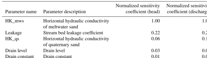
sequen-Table 1. List of parameters included for estimation, including their normalized sensitivity coefficients to head and discharge observations,
respectively.
Normalized sensitivity Normalized sensitivity Parameter name Parameter description coefficient (head) coefficient (discharge)
HK_mws Horizontal hydraulic conductivity 1.00 1.00
of meltwater sand
Leakage Stream bed leakage coefficient 0.22 0.29
HK_qs Horizontal hydraulic conductivity 0.06 0.11
of quaternary sand
Drain level Drain level 0.03 0.07
Drain constant Drain constant 0.01 0.04
tially decreased, which helps maintain a spread in the ensem-ble of state variaensem-bles and avoid an ensemensem-ble collapse.
The hydraulic conductivities of meltwater sand and qua-ternary sand are included. Despite being hydrogeological pa-rameters related to the groundwater module of the model, these are, as evident from Table 1, also sensitive to the dis-charge observations. Also included are the drain level and drain time constant, which control the amount and dynam-ics of groundwater drained to the nearest stream once the groundwater table exceeds the drain level and are as such particularly important for drain flow. The leakage coefficient, which is important with respect to base flow, is another cou-pling parameter, which represents the hydraulic properties of the thin layer of the sediments at the bottom of the stream.
Four of the five estimated parameters, the hydraulic con-ductivities of meltwater sand and quaternary sand, as well as the stream bed leakage coefficient and the drain time constant were transformed logarithmically in the filter as the expected parameter uncertainty is expected to span several decades, with drain level being the only parameter not transformed. As commonly practiced in calibration of hydrological mod-els, the horizontal hydraulic conductivities were tied to the vertical hydraulic conductivities of the respective geological units at a fixed ratio of 10 to 1.
The parameter updates are dampened by a factor of 0.1, meaning that only a tenth of the update (as determined by the filter) is used. This is based on Hendricks Franssen et al. (2008), who showed that damping improves the parameter estimation process.
2.4 Twin test setup
This study uses a twin test in which observations are gener-ated by extracting selected state values from a forward run (“true” model), and adding normally distributed noise to em-ulate typical real-world observation errors. For comparison, the results of a model similar to the true model, but with per-turbed initial parameter values, will be shown. This shows the states of the model if no state updating or parameter es-timation is applied and will in the following be denoted the
base model. The parameter values used to generate the base model and the true model can be seen in Table 2.
2.5 Model noise
Model noise is added to the ensemble through the forcings, i.e., precipitation and reference evapotranspiration, and the parameters. Noise on forcings is added as a Gaussian noise with a standard deviation of 20 % of the observed value, while no spatial correlation of the noise is considered.
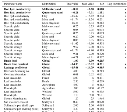
Noise is added to a large number of model parameters re-lating to all model processes as seen in Table 2. In total, noise is added to 66 parameters, only 5 of which are es-timated. Adding noise to parameters that are not estimated helps maintain the spread of the ensemble even as the spread of the estimated parameters is reduced.
The noise added to both forcings and parameters is based on experience with uncertainty in real data and parameters. The magnitude of parameter uncertainty is for many param-eters well understood, as sensitivity analysis and calibration has been performed on several hydrological models, includ-ing the Karup catchment model (Refsgaard, 1997). Correla-tion in parameter values is only included where this is widely accepted to exist and easily quantifiable (i.e., horizontal and vertical hydraulic conductivity). The noise added to the forc-ings represents a significant simplification of the understand-ing of forcunderstand-ing uncertainty, which is likely to be highly cor-related both temporally and spatially. A better description of the correlation in forcing noise would most likely have re-sulted in better description of the error covariances, which currently is determined based on the difference in model be-havior between the ensemble members, and thereby better filter performance in terms of distributing the state updates. However, spatially and temporally correlated ensembles of forcings are difficult to generate and outside the scope of this study.
2.6 Data availability
[image:6.612.102.493.97.207.2]Table 2. List of parameters perturbed to create the true model and to add noise to the filter ensemble. Parameters in bold are included in
the parameter estimation. Parameters with very low sensitivity were omitted. Parameters are perturbed using Gaussian noise with standard deviation (SD) shown in the table.
Parameter name Distribution True value base value SD Log transformed
Hor. hyd. conductivity Meltwater sand −8.52 −7.60 0.818 x
Hor. hyd. conductivity Quaternary sand −6.21 −7.01 1.151 x
Hor. hyd. conductivity Clay −15.42 −15.42 0.194 x
Hor. hyd. conductivity Mica sand −11.74 −11.74 0.201 x
Hor. hyd. conductivity Mica clay/sand −16.34 −16.34 0.213 x
Specific yield Meltwater sand 0.25 0.25 0.025
Specific yield Clay 0.05 0.05 0.004
Specific yield Quaternary sand 0.25 0.25 0.023
Specific yield Mica sand 0.20 0.20 0.022
Specific yield Mica clay/sand 0.05 0.05 0.005
Specific storage Meltwater sand −11.62 −9.90 0.308 x
Specific storage Clay −9.57 −9.90 0.335 x
Specific storage Quaternary sand −11.74 −9.90 0.318 x
Specific storage Mica sand −9.21 −9.90 0.320 x
Specific storage Mica clay/sand −6.21 −9.21 0.367 x
Drain level Global −1.00 −0.90 0.215
Drain time constant Global −14.33 −15.02 0.381 x
Leakage coefficient Global −15.48 −14.79 0.885 x
Overland Manning no. Global 4.00 5 0.213
Overland detention Global 0.01 0.02 0.001
Leaf area index Forest 5.00 6 0.431
Leaf area index Heath 2.50 2 0.209
Leaf area index Agriculture 4.00 5 0.413
Root depth Agriculture 900 1000 43.87
Leaf area index Wetland 5.00 6 0.435
Root depth Wetland 710 700 98.91
Stream Manning no. Global 20 25 1.964
Sat. moisture content Soil type 1 0.40 0.40 0.020
Soil matric pot. (field cap) Soil type 1 2.00 2.00 0.088
Soil matric pot. (wilting point) Soil type 1 4.20 4.20 0.168
Sat. hyd. conductivity Soil type 1 −11.18 −11.18 0.345 x
“35 obs” contains observations in all the locations where actual (i.e., real-world) observations are also available and presents an extensive spatial coverage of observations, with observations located in between almost all the branches of the river network and with many of the observations located in neighboring model grid cells. The spatial distribution “8 obs” is a subset of “35 obs” and represents a less exten-sive coverage of observations and with significantly fewer observations than “35 obs”. Moreover, “2 obs” is a subset of “8 obs” and contains only two observations located approxi-mately halfway downstream of the Karup River, and as such represents a scenario in which the spatial coverage of obser-vations is poor. Finally, “0 obs” (not depicted in the figure) represents a scenario in which no groundwater head obser-vations are available. Discharge obserobser-vations are made avail-able in five locations (see Fig. 1), two of which are on the main river branch (one at the catchment outlet and one ap-proximately halfway downstream) with the remaining obser-vations located on the northwestern tributary. Note that the
distribution names only describe the groundwater head ob-servations and that stream discharge obob-servations are always assimilated unless otherwise is stated in the scenario name (see Sect. 2.7).
Herschy (1999). This means that discharge measurement er-rors increase in peak flow situations and are larger for down-stream locations, while the measurement error of head is not related to the location or the observed value.
The states and parameters are updated every time ground-water head observations, i.e., every 28 days, and the daily discharge observations available in between updates are as-similated asynchronously. Tests have shown that the length of the assimilation window is of little importance and there-fore no other assimilation window was tested.
2.7 Scenarios
This study will consist of four scenarios, with varying avail-ability of discharge observations and with and without pa-rameter estimation. In all four scenarios groundwater head data are assimilated.
InclParInclQ: the primary scenario in this study, in which discharge observations are assimilated and parameters are es-timated, constitutes the most complex scenario. Estimating parameters makes the updates more nonlinear compared to stand-alone state updating, and assimilating discharge obser-vations can be expected to require more ensemble members due to the complex relationship between stream discharge and groundwater head.
InclParNoQ: this scenario includes parameter estimation but excludes discharge observations (stream discharge and water level are still included in the state vector). This means that the update of groundwater head, stream discharge and stream water level as well as the parameter estimation is based only on head observations.
NoParInclQ: this scenario includes the assimilation of dis-charge observations but excludes parameter estimation. This way, the influence of differing parameter sets is removed, al-lowing the direct results of updating the states to be seen.
NoParNoQ: this scenario excludes both the assimilation of discharge observations and parameter estimation. The sim-plest of the included scenarios, this scenario, when compared to scenario NoParInclQ illustrates the value of discharge ob-servations on state updating.
2.8 Performance indicators
The performance of the filter will be evaluated based on three indicators:
– mean root mean square error of hydraulic head for the entire domain (every model grid), calculated based on the mean of the ensemble at each time step (12 h time steps) and the true model state. Hereafter denoted head RMSE;
– mean root mean square error of discharge in all grid points in the river network model, calculated based on the mean of the ensemble at each time step (2 h time steps) and the true model state. Hereafter denoted
dis-charge RMSE. Note that this indicator inadvertently is dominated by downstream grid points with higher flow; – the convergence of estimated parameters to the true value, including the spread and mean of the ensemble of parameters.
3 Results and discussion 3.1 Localization tuning
Tuning of the localization algorithm is carried out using a scenario in which two hydraulic head observations and all five discharge observations are available. An ensemble size of 50 is used, as experience had shown that this ensemble size resulted in significant spurious correlation with this number of observations.
The head RMSE as a function of the two localization con-stants can be seen in Fig. 3. Based on these results, constant values ofaandbof 2 are used in the remainder of this study. Due to the computational time required, only integer values of the constants are tested, although it may have been possi-ble to fine-tune the localization algorithm by using fractions. Localization using distance-based localization was ana-lyzed with varying localization distances and compared to using adaptive localization and no localization, as seen in Fig. 3. Overall localization distances of 20 and 10 km that apply to both the groundwater domain and the stream do-main were tested. Compared to using no localization, a small increase in head RMSE is obtained in the case of 20 km lo-calization distance, whereas a significant increase in head RMSE is seen when a localization distance of 10 km is used, which may be explained by true correlation (at a distance of more than 20 or 10 km) being removed from the filter. Simul-taneously, spurious correlation occurring within the specified radii of the observations is not removed by this type of local-ization, which may lead to increases in head RMSE. Com-pared to adaptive localization worse results are obtained, and it is clear that simple distance-based localization with local-ization distances that apply to both groundwater variables and stream variables is not sufficient. It should be noted that the distance-based localization method applied does not dis-tinguish between model processes and that the localization distance also applies to the cross-correlation between the dif-ferent state variables (i.e., groundwater observations are lo-calized with the described distance with regards to stream variables and vice versa).
35 obs 8 obs 2 obs
Figure 2. Spatial distributions of observations. Dots and crosses respectively denote groundwater hydraulic head and stream discharge
[image:9.612.310.545.258.357.2]observation locations, respectively.
Figure 3. Head RMSE as a function of the adaptive localization
constantsaandb(a) and head RMSE using different localization
methods (b).
there is no update across model processes and the two model states (groundwater and stream) are therefore updated inde-pendently from each other. As Fig. 3 shows, both scenarios led to a reduction in head RMSE compared to not using lo-calization, yet head RMSE is still significantly higher than for the scenario with adaptive localization.
The effect of localization becomes clear when studying the time series of head RMSE (Fig. 4). Using no localization, the spurious correlations become dominant, as evident from the regular spikes visible in the dark blue line in Fig. 4. Using the distance-based localization method with 20 km localiza-tion radius does little to remove the spikes (and by extension, the spurious correlation), and a localization radius of 10 km only exacerbates them. Using differentiated localization radii for intra- and cross-process correlation removes a significant part of the spurious correlation with 0 km radius significantly outperforming a 5 km radius. However, a few spikes do per-sist and, compared to the adaptive localization, the decrease in head RMSE during some updates is not as big, suggesting that real correlation is removed.
The lower graph of Fig. 4, which shows the discharge RMSE as a function of time, illustrates why spurious corre-lation is a particular problem for discharge modeling. While the filter can reduce the discharge RMSE to almost zero at the updating time, peaks in the RMSE often appear in the time step immediately after the update. These peaks are the results of spurious correlation in the groundwater manifest-ing itself in the discharge and are due to the nature of the
Figure 4. Head (a) and discharge (b) RMSE for the entire model
domain as a function of time with different types of localization applied. Note that only the discharge RMSE for the year 1972 is shown.
groundwater–streamflow interaction. Spurious correlation in groundwater appears where little real correlation with the ob-servation points is present, which makes the grid cells that exchange water with the stream more sensitive than others. The dynamics of these cells are significantly different from the slow changing dynamics of most groundwater model cells, and any change in the interaction cells are reflected in the streamflow. Put simply, a change in the groundwater head of a few centimeters is barely noticeable in most grid cells, but may result in a significant change in the streamflow if the change is found in the grid cells that controls the interaction with the streamflow.
[image:9.612.51.284.258.310.2]Figure 5. Mean localization weight derived from the adaptive
local-ization algorithm for different observation locations and observation types. Two groundwater observations and two stream discharge ob-servations are included – magenta crosses indicate the observation locations. The two left columns show localization weights for the two groundwater head observations, the third and fourth columns show localization weights for the two discharge observations. An example of the localization weights as obtained using the distance-based localization method, with a localization distance of 10 km, is included for comparison on the right.
the distribution of localization weights appears to primarily depend on the branch on which the observation is located. The most downstream observation (at the model outlet) has the highest localization weights on the main branch of the network while the observation located on the tributary has the highest weights on that tributary (and on its tributaries). For both observations there is an alternation between high-and medium- to low-localization weights visible in the fig-ure, which is a result of the alternation between discharge and water level calculation used in the model. The adaptive local-ization algorithm assigns a lower weight to water level vari-ables than to discharge varivari-ables due to the fact that discharge is what is being observed. One could think that this could lead to some discrepancies in the stream network states after updates, due to improper discharge–water level relations, but no effects (i.e., post update instability or state fluctuations) of this were seen, leading to the conclusion that the model is able to adjust any discrepancies there might be quickly after the states have been updated.
3.2 InclParInclQ
Head RMSE as a function of ensemble size for the scenario InclParInclQ can be seen in Fig. 6. Using 35 observations and no adaptive localization, a small improvement in head RMSE is seen when increasing the ensemble size from 25 to 50, but no change is seen when increasing from 50 to 100, and it appears that an ensemble size of 50 is sufficient in this case. When applying localization, almost no improvement is seen when increasing the ensemble size, suggesting that an ensemble size of 25 (or even less) is sufficient. Reducing the number of observations to 8, an improvement is seen when increasing the ensemble size from 25 to 50, 100 and even 200, with the largest improvement achieved when
increas-Figure 6. Head RMSE (a) and discharge RMSE (b) as a function
of ensemble size in the InclParInclQ scenario for different numbers of groundwater head observations.
[image:10.612.50.285.68.178.2]spa-tial discretization of the model, and larger ensemble sizes are not realistic for practical applications. Using localization, the improvement seen when increasing the ensemble size is very small, and a small increase in head RMSE is even seen when increasing the ensemble size from 50 to 100, suggesting that 50 ensemble members are sufficient in this case. Using two or no head observations also results in improvement when in-creasing the ensemble size to 200. Using localization results in improvement in both scenarios but, even with localization applied, an ensemble size of 200 may not be sufficient.
The results show that the ensemble size needed depends strongly on the number of observations available. With fewer observations, the information from the observations needs to be spread further spatially, and the small correlation that ex-ists relatively far from an observation needs to be estimated well, which requires more ensemble members. With a more extensive spatial coverage of observations, the small corre-lation of an observation and a distant model grid point be-comes less important, as there is more likely to be another observation closer with a higher correlation which is better estimated with fewer ensemble members to estimate. As a result, a larger ensemble size is required when the spatial coverage of observations is poor. Localization removes the spurious correlation and thus improves the performance at lower ensemble sizes or lower observation numbers but does not affect the sampling error itself. As a result, very large en-semble sizes are necessary when very few observations are available, even if localization is applied.
In terms of discharge RMSE (the lower graph in Fig. 6), the relationship between ensemble size and RMSE is a bit more unclear, due to spurious correlation being significant in most cases except “35 obs”. The presence of spurious corre-lations depends strongly on the sampling of both parameters and model forcing noise and is by nature random. As such, a clear trend in RMSE as a function of ensemble size cannot always be expected when spurious correlation is a significant source of error. However, a general improvement is observed when using localization in most cases, with a significant im-provement observed in the “0 obs” case, where spurious cor-relations are also most apparent.
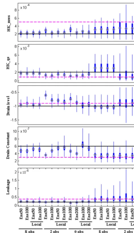
As Fig. 7 shows, the performance of parameter estimation is related to the ensemble size and the number of observa-tions as well as to the application of localization. When as-similating eight observations, a slight improvement in the es-timation of the drain level and drain constant is observed, while little or no improvement is observed when estimating the remaining parameters. The improvement with localiza-tion is more pronounced when only two or no head obser-vations are assimilated, where an improvement can also be observed when the ensemble size is increased.
3.3 InclParNoQ
[image:11.612.309.545.65.473.2]The head RMSE as a function of ensemble size for the sce-nario InclParNoQ can be seen in the leftmost graphs in Fig. 8.
Figure 7. Spread of estimated parameters at the final update. Thin
blue lines show the total spread of the ensemble and thick blue lines show the 25th and 75th percentiles. Dots show the mean of the en-semble. The horizontal lines show the true parameter value (black line) and the base parameter value (magenta line).
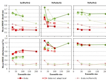
Figure 8. Head RMSE (top) and discharge RMSE (bottom) as a function of ensemble size for three of the scenarios. For comparison, the
dashed lines indicate the head and discharge RMSE of the InclParInclQ scenario (without localization).
for groundwater head updating, discharge observations could be left out, as they result in little or no improvement in the groundwater domain and requires a larger ensemble size.
The discharge RMSE in Fig. 8 shows that clear improve-ments in the discharge RMSE is achieved with the assim-ilation of discharge observations. Both the scenarios with eight observations and with two observations show increas-ing trends with respect to discharge RMSE versus ensemble size, which seems to be related to the estimation of parame-ters, particularly the leakage coefficient which was estimated worse with increasing ensemble size (i.e., the mean of the en-semble of parameter values was offset from the true value). This is presumably done by the filter to optimize the ground-water state but leads to significant biases in the estimated pa-rameter values.
The estimated parameter values can be seen in Fig. 7, which shows that little or no improvement in the estimation of parameters is obtained by increasing the ensemble size or by adding localization. When comparing to the parameter estimation of the InclParInclQ scenario, the estimation of all parameters is clearly worse in InclParNoQ, both in terms of the mean and the spread of the ensemble, underlining the ne-cessity of assimilating discharge observations in integrated hydrological models, if the aim is to estimate parameters. 3.4 NoParInclQ
For the scenario NoParInclQ, the head and discharge RMSE as a function of ensemble size can be seen in the two
not observed in InclParInclQ, as the parameter spread there is sequentially reduced.
When using eight observations, a general decrease in head and discharge RMSE is observed with increasing ensemble size. There is a significant difference when using localiza-tion, with localization increasing the head RMSE and de-creasing the discharge RMSE substantially. The decrease in discharge RMSE is explained by the removal of spurious cor-relation, which can cause significant problems for the dis-charge in particular (see Sect. 3.1). The general increase in head RMSE may be explained by the trade-off effect shifting between the groundwater and the discharge observations.
In both cases when using either eight or two observations, the effect on the head RMSE is relatively small. This is most likely due to the slow changing dynamics of groundwater, which means that the groundwater head is well constrained and does not deviate significantly from the “true” ground-water head in between updates. The discharge, on the other hand, changes very rapidly, and the effect of updating the discharge at a specific time will quickly disappear after the model is started again. Adding to this is the problem with spurious correlation and its relevance to discharge model-ing (see Sect. 3.1) which often results in very high discharge RMSE and makes direct comparison of the discharge RMSE between scenarios difficult.
3.5 NoParNoQ
The head and discharge RMSE when parameter estimation and discharge observations are omitted can be seen in the two rightmost graphs of Fig. 8. Both when using two obser-vations and eight obserobser-vations, the resulting changes in head and discharge RMSE with increasing ensemble size are very small. Likewise, the benefit of using localization is negligi-ble. This may be explained by the updating being much more linear than in any of the other scenarios, thus reducing the need for a large ensemble size.
When comparing the NoParNoQ results with the NoParIn-clQ results, it becomes clear that the impact of assimilating discharge (without estimating parameters) is small with re-spect to both head RMSE and discharge RMSE both in the case of using eight observations and two observations. How-ever, the trade-off issue does not exist in the NoParNoQ sce-nario, causing this scenario to perform better with respect to head RMSE when two observations are used.
4 Conclusions
This study investigated the impact of localization and en-semble size when applying data assimilation to a coupled surface–subsurface model, considering different types and varying amount of observation data and parameter estima-tion.
The adaptive localization method used in this study was in many cases able to reduce the required ensemble size signif-icantly. The method resulted in a complex distribution of lo-calization weights in both domains of the model (groundwa-ter and streamflow) that depended heavily on the geology and the position of the observation relative to the stream network. This distribution could not be obtained using the common distance-based methods, and direct comparison of the adap-tive localization and distance-based localization also showed that adaptive localization outperformed distance-based local-ization with respect to head RMSE. Adaptive locallocal-ization is not only easily implemented in the ETKF, it also automat-ically ensures that the cross-process correlation is localized differently than the intra-process correlation, making it par-ticularly suitable for data assimilation in coupled surface– subsurface models. Others have encountered the problem with cross-process correlation, notably Zupanski (2013), Li et al. (2013) and Wanders et al. (2014), although no definitive solution to the problem has been presented. Adaptive local-ization, such as the method applied in this study, may be one possible solution.
When assimilating both groundwater head observations and estimating parameters, localization and large ensemble sizes are important due to the nonlinearity of the state and parameter updates. This tendency is increasingly pronounced with decreasing number of observations assimilated due to the small correlations between observations and model states being more important when the spatial distribution of ob-servations is poor. Excluding discharge obob-servations reduces the benefits of localization and increasing ensemble size, as does the exclusion of parameter estimation. When excluding both discharge observation assimilation and parameter esti-mation applying localization or increasing the ensemble size from 25 to 50, 100 or 200 has almost no effect on the filter performance. The effects of increasing ensemble size in hy-drological modeling has previously been studied (Chen et al, 2013; Xie and Zhang, 2010), with findings similar to the ones of this study. Both studies found that increases in ensemble size improved filter performance, e.g., Xie and Zhang (2010) increased the ensemble size to 1000 and still observed im-provements. However, neither of the studies related the en-semble size to the amount of observations assimilated or to the estimation of parameters.
Like with state updating, estimation of parameters was pri-marily improved by an increasing ensemble size when dis-charge observations were assimilated. With disdis-charge obser-vations assimilated, clear improvements in parameter estima-tion were observed when applying localizaestima-tion, and to some extent when increasing the ensemble size (depending on the number of assimilated head observations). However, no im-provement was observed when applying localization or in-creasing the ensemble size when discharge observations were not assimilated.
of parameters, as well as on the available number of obser-vations. A large ensemble size is necessary when discharge observations are assimilated, parameters are estimated and few observations are available, while a significantly smaller ensemble size is sufficient when only groundwater head is assimilated and updated. However, the best overall filter performance (i.e., a combination of groundwater head and streamflow modeling) is found when discharge observations are assimilated and parameters are estimated. While the findings of this study could to a certain extent be derived intuitively, this is to our knowledge the first time that they have been quantified and documented in integrated hydrological modeling.
Edited by: V. Andréassian
References
Albergel, C., Rüdiger, C., Pellarin, T., Calvet, J.-C., Fritz, N., Frois-sard, F., Suquia, D., Petitpa, A., Piguet, B., and Martin, E.: From near-surface to root-zone soil moisture using an exponential fil-ter: an assessment of the method based on in-situ observations and model simulations, Hydrol. Earth Syst. Sci., 12, 1323-1337, doi:10.5194/hess-12-1323-2008, 2008.
Anderson J. L.: Exploring the need for localization in en-semble data assimilation using a hierarchical enen-semble filter, Physica D: Nonlinear Phenomena, 230, 99–111, doi:10.1016/j.physd.2006.02.011, 2007.
Anderson, J. L. and Anderson, S. L.: A Monte Carlo implementa-tionof the nonlinear filtering problem to produce ensemble as-similations and forecasts, Mon. Weather Rev. 127, 2741–2758, 1999.
Bishop, C. H. and Hodyss, D.: Ensemble covariances adaptively lo-calized with ECO-RAP. Part 1: Tests on simple error models, Tellus, 61A, 84–96, 2009.
Bishop, C. H., Etherton, B. J., and Majumdar, S. J.: Adaptive sam-pling with the ensemble transform kalman filter. part I: Theoret-ical aspects, Mon. Weather Rev., 129, 420–436, 2001.
Camporese, M., Paniconi, C., Putti, M., and Salandin, P.: Ensem-ble Kalman filter data assimilation for a process-based catchment scale model of surface and subsurface flow, Water Resour. Res., 45, W10421, doi:10.1029/2008WR007031, 2009.
Chen, H., Yang, D., Hong, Y., Gourley, J .J., and Zhang, Y.: Hydro-logical data assimilation with the Ensemble Square-Root-Filter: Use of streamflow observations to update model states for real-time flash flood forecasting, Adv. Water Resour., 59, 209–220, doi:10.1016/j.advwatres.2013.06.010, 2013.
Craig, H., Bishop, B. J. E., and Sharanya, J. M.: Adaptive Sampling with the Ensemble Transform Kalman Filter. Part I: Theoretical Aspects, Mon. Weather Rev., 129, 420–436, 2001.
Drécourt, J.-P., Madsen, H., and Rosbjerg, D.: Bias aware Kalman filters: Comparison and improvements, Adv. Water Resour., 29, 707–718, doi:10.1016/j.advwatres.2005.07.006, 2005.
Fertig, E. J., Hunt, B. R., Ott, E., and Szunyogh, I.: Assimilat-ing non-local observations with a local ensemble Kalman filter, Tellus A, 59, 719–730, doi:10.1111/j.1600-0870.2007.00260.x, 2007
Graham, D. N. and Butts, M. B.: Flexible, integrated watershed modelling with MIKE SHE, in: Watershed Models, edited by: Singh, V. P. and Frevert, D. K., 245–272, CRC Press, ISBN: 0849336090, Boca Raton, Florida, USA, 2005.
Greve, M. H., Greve, M. B., Bøcher, P. K., Balstrøm, T., Breuning-Madsen, H., and Krogh, L.: Generating a Danish raster-based topsoil property map combining choropleth maps and point in-formation, Geografisk Tidsskrift, 107, 1–12, 2007.
Harlim, J. and Hunt, B. R.: Local Ensemble Transform Kalman Filter: An Efficient Scheme for Assimilating Atmospheric Data, preprint (2005).
Hendricks Franssen, H. J. and Kinzelbach, W.: Real-time groundwater flow modeling with the Ensemble Kalman Fil-ter: Joint estimation of states and parameters and the fil-ter inbreeding problem, Wafil-ter Resour. Res., 44, W09408, doi:10.1029/2007WR006505, 2008.
Hendricks Franssen, H. J., Kaiser, H. P., Kuhlmann, U., Bauser, G., Stauffer, F., Muller, R., and Kinzelbach, W.: Operational real-time modeling with ensemble Kalman filter of variably saturated subsurface flow including stream-aquifer interaction and parameter updating, Water Resour. Res., 47, W02532, doi:10.1029/2010WR009480, 2011.
Herschy, R. W.: Hydrometry – Principles and Practices, 2nd Edn., Wiley & Sons Ltd, Hoboken, New Jersey, USA, 1999.
Hunt, B., Kostelich, E., and Syzunogh, I.: Efficient data assimilation for spatiotemporal chaos: A local ensemble transform Kalman filter, Physica D, 230, 112–126, 2007.
Juston, J., Seibert, J., and Johansson, P.-O.: Temporal sampling strategies and uncertainty in calibrating a conceptual hydrolog-ical model for a small boreal catchment, Hydrol. Process., 23, 3093–3109, DOI:10.1002/hyp.7421, 2009.
Kristensen, K. J. and Jensen, S. E.: A model of estimating ac-tual evapotranspiration from potential evapotranspiration, Nordic Hydrol., 6, 170–188, 1975.
Li, Y., Ryu, D., Western, A. W., and Wang, Q. J.: Assimilation of stream discharge for flood forecasting: The benefits of account-ing for routaccount-ing time lags, Water Resour. Res., 49, 1887–1900, doi:10.1002/wrcr.20169, 2013.
Liu, Y. and Gupta, H. V.: Uncertainty in hydrologic modeling: To-ward an integrated data assimilation framework, Water Resour. Res., 43, W07401, doi:10.1029/2006WR005756, 2007. Madsen, H.: Parameter estimation in distributed hydrological
catch-ment modelling using automatic calibration with multiple ob-jectives, Adv. Water Resour., 26, 205–216, doi:10.1016/S0309-1708(02)00092-1, 2003.
Moradkhani, H., Sorooshian, S., Gupta, H. V., and Houser, P.: Dual State-Parameter Estimation of Hydrological Models using En-semble Kalman Filter, Adv. Water Resour., 28, 135–147, 2005. Miyoshi, T.: An adaptive covariance localization method with the
LETKF (presentation), 14th Symposium on Integrated Observ-ing and Assimilation Systems for the Atmosphere, Oceans, and Land Surface (IOAS-AOLS) (recorded presentation), 2010. Nie, S., Zhu, J., and Luo, Y.: Simultaneous estimation of land
sur-face scheme states and parameters using the ensemble Kalman filter: identical twin experiments, Hydrol. Earth Syst. Sci., 15, 2437–2457, doi:10.5194/hess-15-2437-2011, 2011.
ensemble Kalman filter for atmospheric data assimilation, Tellus A, 56, 415–428, doi:10.1111/j.1600-0870.2004.00076.x, 2004. Refsgaard, J. C.: Parametrisation, calibration and validation of
dis-tributed hydrological models, J. Hydrol., 198, 69–97, 1997. Sakov, P. and Bertino, L.: Relation between two common
localisa-tion methods for the EnKF, Comput. Geosci., 15, 225–237, 2011. Sakov, P., Evensen, G., and Bertino, L.: Asynchronous data assim-ilation with the EnKF, Tellus, 62A, 24–29, doi:10.1111/j.1600-0870.2009.00417.x, 2010.
Shi, Y., Davis, K. J., Zhang, F., Duffy, C. J., and Yu, Z.: Parameter Estimation of a Physically-Based Land Sur-face Hydrologic Model Using the Ensemble Kalman Filter: A Synthetic Experiment, Water Resour. Res., 50, 706–724, doi:10.1002/2013WR014070, 2014.
Vrugt, J. A., Diks, C. G. H., Gupta, H. V., Bouten, W., and Verstraten, J. M.: Improved treatment of uncertainty in hydro-logic modeling: Combining the strengths of global optimiza-tion and data assimilaoptimiza-tion, Water Resour. Res., 41, W01017, doi:10.1029/2004WR003059, 2005.
Wanders, N., Karssenberg, D., de Roo, A., de Jong, S. M., and Bierkens, M. F. P.: The suitability of remotely sensed soil moisture for improving operational flood forecasting, Hydrol. Earth Syst. Sci., 18, 2343–2357, doi:10.5194/hess-18-2343-2014, 2014.
Xie, X. and Zhang, D.: Data assimilation for distributed hydrolog-ical catchment modeling via ensemble Kalman filter, Adv. Wa-ter Resour., 33, 678–690, doi:10.1016/j.advwatres.2010.03.012, 2010.