Exploring water cycle dynamics by sampling multiple stable water isotope pools in a developed landscape in Germany

Exploring water cycle dynamics by sampling multiple stable water

isotope pools in a developed landscape in Germany

Natalie Orlowski1,2, Philipp Kraft1, Jakob Pferdmenges1, and Lutz Breuer1,3

1_{Institute for Landscape Ecology and Resources Management (ILR), Research Centre for BioSystems, Land Use and}

Nutrition (iFZ), Justus Liebig University Gießen, Gießen, Germany

2_{Global Institute for Water Security, University of Saskatchewan, Saskatoon, Canada}

3_{Centre for International Development and Environmental Research, Justus Liebig University Gießen, Gießen, Germany} Correspondence to:N. Orlowski ([email protected])

Received: 5 November 2014 – Published in Hydrol. Earth Syst. Sci. Discuss.: 6 February 2015 Revised: 27 July 2016 – Accepted: 16 August 2016 – Published: 20 September 2016

Abstract.A dual stable water isotope (δ2H andδ18O) study was conducted in the developed (managed) landscape of the Schwingbach catchment (Germany). The 2-year weekly to biweekly measurements of precipitation, stream, and groundwater isotopes revealed that surface and groundwa-ter are isotopically disconnected from the annual precipita-tion cycle but showed bidirecprecipita-tional interacprecipita-tions between each other. Apparently, snowmelt played a fundamental role for groundwater recharge explaining the observed differences to precipitationδvalues.

A spatially distributed snapshot sampling of soil water iso-topes at two soil depths at 52 sampling points across different land uses (arable land, forest, and grassland) revealed that topsoil isotopic signatures were similar to the precipitation input signal. Preferential water flow paths occurred under forested soils, explaining the isotopic similarities between top- and subsoil isotopic signatures. Due to human-impacted agricultural land use (tilling and compression) of arable and grassland soils, water delivery to the deeper soil layers was reduced, resulting in significant different isotopic signatures. However, the land use influence became less pronounced with depth and soil water approached groundwaterδvalues. Seasonally tracing stable water isotopes through soil profiles showed that the influence of new percolating soil water de-creased with depth as no remarkable seasonality in soil iso-topic signatures was obvious at depths > 0.9 m and constant values were observed through space and time. Since classic isotope evaluation methods such as transfer-function-based mean transit time calculations did not provide a good fit be-tween the observed and calculated data, we established a

hy-drological model to estimate spatially distributed groundwa-ter ages and flow directions within the Vollnkirchener Bach subcatchment. Our model revealed that complex age dynam-ics exist within the subcatchment and that much of the runoff must has been stored for much longer than event water (av-erage water age is 16 years). Tracing stable water isotopes through the water cycle in combination with our hydrologi-cal model was valuable for determining interactions between different water cycle components and unravelling age dy-namics within the study area. This knowledge can further improve catchment-specific process understanding of devel-oped, human-impacted landscapes.

1 Introduction

under-standing results from studies in forested catchments. Spatio-temporal studies of stream water in developed, agricultur-ally dominated, and managed catchments are less abundant. This is partly caused by damped stream water isotopic sig-natures excluding traditional hydrograph separations in low-relief catchments (Klaus et al., 2015). Unlike the distinct watershed components found in steeper headwater counter-parts, lowland areas often exhibit a complex groundwater– surface-water interaction (Klaus et al., 2015). Sklash and Far-volden (1979) showed that groundwater plays an important role as a generating factor for storm and snowmelt runoff pro-cesses. In many catchments, streamflow responds promptly to rainfall inputs but variations in passive tracers such as water isotopes are often strongly damped (Kirchner, 2003). This indicates that storm runoff in these catchments is domi-nated mostly by “old water” (Buttle, 1994; Neal and Rosier, 1990; Sklash, 1990). However, not all old water is the same (Kirchner, 2003). This catchment behaviour was described by Kirchner (2003) as the old-water paradox. Thus, there is evidence of complex age dynamics within catchments and much of the runoff is stored in the catchment for much longer than event water (Rinaldo et al., 2015). Still, some of the physical processes controlling the release of old water from catchments are poorly understood and roughly modelled, and the observed data do not suggest a common catchment be-haviour (Botter et al., 2010). However, old-water paradox behaviour was observed in many catchments worldwide, but it may have the strongest effect in agriculturally managed catchments, where surprisingly only small changes in stream chemistry have been observed (Hrachowitz et al., 2016).

Moreover, almost all European river systems were al-ready substantially modified by humans before river ecol-ogy research developed (Allan, 2004). Through changes in land use, land cover, irrigation, and draining, agriculture has substantially modified the water cycle in terms of both quality and quantity (Gordon et al., 2010) as well as hy-drological functioning (Pierce et al., 2012). Hrachowitz et al. (2016) recently stated the need for a stronger linkage be-tween catchment-scale hydrological and water quality com-munities. Further, McDonnell et al. (2007) concluded that we need to figure out a way to embed landscape heterogeneity or the consequence of the heterogeneity (i.e. of agriculturally dominated and managed catchments) into models as current-generation catchment-scale hydrological and water quality models are poorly linked (Hrachowitz et al., 2016).

One way to better understand catchment behaviour and the interaction among the various water sources (surface, sub-surface, and groundwater) and their variation in space and time is a detailed knowledge about their isotopic composi-tion. In principal, isotopic signatures of precipitation are al-tered by temperature, amount (or rainout), continental, altitu-dinal, and seasonal effects. Stream water isotopic signatures can reflect precipitation isotopic composition and, moreover, dependent on discharge variations, be affected by season-ally variable contributions of different water sources such as

bidirectional water exchange with the groundwater body dur-ing baseflow or high event-water contributions durdur-ing storm flow (Genereux and Hooper, 1998; Koeniger et al., 2009). Precipitation falling on vegetated areas is partly intercepted by plants and re-evaporated isotopically fractionated. The remaining throughfall infiltrates slower and can be affected by evaporation resulting in an enrichment of heavy isotopes, particularly in the upper soil layers (Gonfiantini et al., 1998; Kendall and Caldwell, 1998). In the soil, specific isotopic profiles develop, characterized by an evaporative layer near the surface. The isotopic enrichment decreases exponentially with depth, representing a balance between the upward con-vective flux and the downward diffusion of the evaporative signature (Barnes and Allison, 1988). In humid and semi-humid areas, this exponential decrease is generally inter-rupted by the precipitation isotopic signal. Hence, the combi-nation of the evaporation effect and the precipitation isotopic signature determine the isotope profile in the soil (Song et al., 2011). Once soil water reaches the saturated zone, this isotope information is finally transferred to the groundwater (Song et al., 2011). Soil water can therefore be seen as a link between precipitation and groundwater, and the dynamics of isotopic composition in soil water are indicative of the pro-cesses of precipitation infiltration, evaporation of soil water, and recharge to groundwater (Blasch and Bryson, 2007; Song et al., 2011).

Figure 1.Maps show(a)the location of the Schwingbach catchment in Germany,(b)the main monitoring area,(c)the land use, elevation, and instrumentation,(d)the locations of the snapshot as well as the seasonal soil samplings,(e)soil types, and(f)geology of the Schwingbach catchment including the Vollnkirchener Bach subcatchment boundaries.

2 Materials and methods 2.1 Study area

The research was carried out in the Schwingbach catch-ment (50◦3004.2300N, 8◦3302.8200E) (Germany) (Fig. 1a). The Schwingbach and its main tributary the Vollnkirchener Bach are low mountainous creeks and have an altitudinal dif-ference of 50–100 m over a 5 km distance (Perry and

distributed along streams, and smaller meadow orchards are located around the villages.

The Schwingbach main catchment is underlain by argilla-ceous shale in the northern parts, serving as aquicludes. Greywacke zones with lydite in the central, as well as lime-stone, quartzite, and sandstone regions in the headwater area provide aquifers with large storage capacities (Fig. 1f). Loess covers Paleozoic bedrock at north- and east-bounded hill-sides (Fig. 1f). Streambeds consists of sand and debris cov-ered by loam and some larger rocks (Lauer et al., 2013). Many downstream sections of both creeks are framed by armour stones (Orlowski et al., 2014). The dominant soil types in the overall study area are Stagnosols (41 %) and mostly forested Cambisols (38 %). Stagnic Luvisols with thick loess layers, Regosol, Luvisols, and Anthrosols are found under agricultural use and Gleysols under grassland along the creeks.

The climate is classified as temperate with a mean an-nual temperature of 8.2◦C. An annual precipitation sum of 633 mm (for the hydrological year 1 November 2012 to 31 October 2013) was measured at the catchment’s climate station (site 13, Fig. 1b). The year 2012 to 2013 was an av-erage hydrometeorological year. For comparison, the climate station Gießen/Wettenberg (25 km north of the catchment) operated by the German Meteorological Service (DWD, 2014) records a mean annual temperature of 9.6◦C and a mean annual precipitation sum of 666±103 mm for the pe-riod 1980–2010. Discharge peaks from December to April (measured by the use of RBC flumes with a maximum peak flow of 114 L s−1, Eijkelkamp Agrisearch Equipment, Gies-beek, NL), and low flows occur from July until November. Substantial snowmelt peaks were observed during Decem-ber 2012 and February 2013. Furthermore, May 2013 was an exceptionally wet month characterized by discharge of 2– 3 mm day−1. A detailed description of runoff characteristics is given by Orlowski et al. (2014).

2.2 Monitoring network and water isotope sampling The monitoring network consists of an automated climate station (site 13, Fig. 1b–c) (Campbell Scientific Inc., AQ5, UK; equipped with a CR1000 data logger), 3 tipping buck-ets, and 15 precipitation collectors, 6 stream water sampling points, and 22 piezometers (Fig. 1b–c). Precipitation data were corrected according to Xia (2006).

Two stream water sampling points (sites 13 and 18) in the Vollnkirchener Bach are installed with trapezium-shaped RBC flumes for gauging discharge (Eijkelkamp Agrisearch Equipment, Giesbeek, NL), and a V-notch weir is located at sampling point 64. RBC flumes and V-notch weir are equipped with Mini-Divers® (Eigenbrodt Inc. & Co. KG, Königsmoor, DE) for automatically recording water lev-els. Discharge at the remaining stream sampling points was manually measured applying the salt dilution method (WTW-cond340i, WTW, Weilheim, DE). The 22

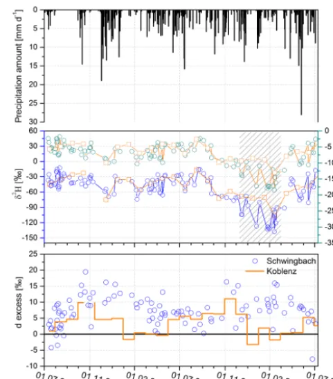
piezome-Figure 2.Temporal variation of precipitation amount, isotopic sig-natures (δ2H andδ18O) including snow samples (grey striped box) of the Schwingbach and GNIP station Koblenz, and d-excess values for the study area compared to monthly d-excess values (July 2011 to July 2013) of GNIP station Koblenz with reference d excess of GMWL (d=10; solid black line).

ters (Fig. 1b) are made from perforated PVC tubes sealed with bentonite at the upper part of the tube to prevent con-tamination by surface water. For monitoring shallow ground-water levels, either combined ground-water level and temperature loggers (Odyssey Data Flow System, Christchurch, NZ) or Mini-Diver®water level loggers (Eigenbrodt Inc. & Co. KG, Königsmoor, DE) are installed. The accuracy of Mini-Diver® is ±5 mm and it is ±1 mm for the Odyssey data logger. For calibration purposes, groundwater levels are additionally measured manually via an electric contact gauge.

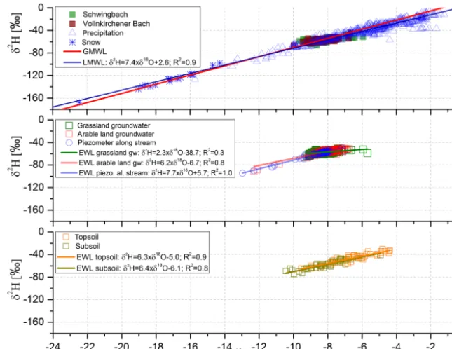
Figure 3.Local meteoric water line for the Schwingbach catchment (LMWL) in comparison to GMWL, including comparisons between precipitation, stream water, groundwater, and soil water isotopic signatures and the respective EWLs.

with three sampling points at each stream (Fig. 1b–c). Since spatial isotopic variations of groundwater among piezome-ters under the meadow were small, samples were collected at three out of eight sampling points under the meadow (sites 3, 6, and 21), five under the arable field (sites 25–29), and four next to the Vollnkirchener Bach (sites 24, 31, 32, and 35) (Fig. 1b). Additionally, a drainage pipe (site 15) lo-cated∼226 m downstream of site 18 was sampled. Accord-ing to IAEA standard procedures, all samples were filled and stored in 2 mL brown glass vials, sealed with a solid lid, and wrapped up with Parafilm®.

2.3 Isotopic soil sampling 2.3.1 Spatial variability

In order to analyse the effect of small-scale characteristics such as distance to stream, topographic wetness index (TWI), and land use on soil isotopic signatures, we sampled a snap-shot of 52 points evenly distributed over a 200 m grid around the Vollnkirchener Bach (Fig. 1d). Soil samples were taken on four consecutive rainless days (1 to 4 November 2011) at elevations of 235–294 m a.s.l. Sampling sites were selected via a stratified, GIS-based sampling plan (ArcGIS, Arc Map 10.2.1, Esri, California, USA), including three classes of TWIs (4.4–6.5; 6.5–7.7; 7.7–18.4), two different distances to the stream (0–121 and 121–250 m), and three land uses (arable land, forest, and grassland), with each class contain-ing the same number of samplcontain-ing points. Samples were

col-Figure 4.Box plots ofδ2H values comparing precipitation, stream, groundwater, and soil isotopic composition at 0.2 and 0.5 m depth (N=52 per depth). Different letters indicate significant differences (p≤0.05).

Figure 5.Dual isotope plot of soil water isotopic signatures at 0.2 and 0.5 m depth compared by land use including precipitation isotope data from 19, 21, and 28 October 2011. Insets: box plots comparingδ2H isotopic signatures between different land use units and precipitation (small letters) in top- and subsoil (capital letters). Different letters indicate significant differences (p≤0.05).

2.3.2 Seasonal isotope soil profiling and isotope analysis

In order to trace the seasonal development of stable water iso-topes from rainfall to groundwater, seven soil profiles were taken in the dry summer season (28 August 2011), seven in the wet winter period (28 March 2013), and two profiles in spring (24 April 2013) under different vegetation cover (arable land and grassland) (Fig. 1d). Soil was sampled from

the soil surface to 2 m depth utilizing a hand auger (Ei-jkelkamp Agrisearch Equipment BV, Giesbeek, DE). More samples were collected near the soil surface since this area is known to have the greatest isotopic variability (Barnes and Allison, 1988).

tem-Figure 6.Seasonalδ2H profiles of soil water (upper panels) and water content (lower panels) for winter (28 March 2013), summer (28 Au-gust 2011), and spring (24 April 2013). Error bars represent the natural isotopic variation of the replicates taken during each sampling campaign. For reference, mean groundwater (grey shaded) and mean seasonal precipitationδ2H values are shown (coloured arrows at the top).

perature of 90◦C following Orlowski et al. (2013). Isotopic signatures of δ18O andδ2H were analysed via off-axis in-tegrated cavity output spectroscopy (OA-ICOS) (DLT-100, Los Gatos Research Inc., Mountain View, USA). Within each isotope analysis three calibrated stable water isotope

Figure 7.Mean daily discharge at the Vollnkirchener Bach (13, 18) and Schwingbach (site 11, 19, and 64) with automatically recorded data (solid lines) and manual discharge measurements (asterisks), temporal variation ofδ2H of stream water in the Schwingbach (site 11, 19, and 64) and Vollnkirchener Bach (site 13, 18, and 94) including moving averages (MAs) for streamflow isotopes.

into the analyser. Then, the first three measurements are dis-carded. The remaining are averaged and corrected for per mil scale linearity following the IAEA laser spreadsheet template (Newman et al., 2009). Following this IAEA standard proce-dure allows for drift and memory corrections. Isotopic ra-tios are reported in per mil (‰) relative to Vienna Standard Mean Ocean Water (VSMOW) (Craig, 1961b). The accuracy of analyses was 0.6 ‰ for δ2H and 0.2 ‰ forδ18O (LGR, 2013). Leaf water extracts typically contain a high fraction of organic contaminations, which might lead to spectral inter-ferences when using isotope ratio infrared absorption spec-troscopy, causing erroneous isotope values (Schultz et al., 2011). However, for soil water extracts there exists no need to check or correct such data (Schultz et al., 2011; Zhao et al., 2011).

2.4 Mean transit time estimation

To understand the connection between the different water cy-cle components in the Schwingbach catchment, mean transit times (MTTs) for both streams as well as from precipitation to groundwater were calculated using FlowPC (Maloszewski and Zuber, 2002). See Appendix A for details about the ap-plied method.

2.5 Model-based groundwater age dynamics

To estimate the age dynamics of the groundwater body in the Vollnkirchener Bach subcatchment, a hydrological model was established on the basis of the conceptual model

pre-sented by Orlowski et al. (2014) and the isotopic measure-ments presented here. Appendix B outlines the modelling concept, model set-up, and its parameterization.

2.6 Statistical analyses

For statistical analyses, we used IBM SPSS Statistics (Version 22, SPSS Inc., Chicago, IL, US) and R (ver-sion Rx64 3.2.2). The R package igraph was utilized for plot-ting (Csardi and Nepusz, 2006). In order to study temporal and spatial variations in meteoric and groundwater, isotope data were tested for normal distribution. Subsequently,ttests or multivariate analyses of variance (MANOVAs) were ap-plied and Tukey’s honest significant difference (HSD) tests were run to determine which groups were significantly dif-ferent (p≤0.05). Event mean values of isotopes in precip-itation, stream, and groundwater were calculated when no spatial variation was observed. Regression analyses were run to determine the effect of small-scale characteristics such as distance to stream, TWI, and land use on soil isotopic signa-tures.

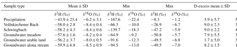
δ2H (‰) δ18O (‰) δ2H (‰) δ18O (‰) δ2H (‰) δ18O (‰)

Precipitation −43.9±23.4 −6.2±3.1 −167.6 −22.4 −8.3 −1.2 5.9±5.7 592 Vollnkirchener Bach −58.0±2.8 −8.4±0.4 −66.3 −10.0 −26.9 −6.7 9.0±2.3 332 Schwingbach −58.2±4.3 −8.4±0.6 −139.7 −18.3 −47.2 −5.9 9.0±2.2 463 Groundwater meadow −57.6±1.6 −8.2±0.4 −64.9 −9.2 −50.8 −5.7 7.9±5.5 375 Groundwater arable land −56.2±3.7 −8.0±0.5 −91.6 −12.3 −49.5 −6.8 1.7±5.0 338 Groundwater along stream −59.9±6.8 −8.5±0.9 −94.5 −13.0 −49.5 −7.0 8.2±1.5 108

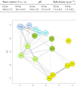
isotope data sets, despite some differences in the exact clus-ter centroid locations. We therefore decided to use randomly selected 80 % of the isotope time series to illustrate our re-sults. In the network map, each node of the network repre-sents an isotope sampling point. The locations of the nodes are based on the first two components (PC1 and PC2). The correlations between isotope time series are represented by the edges connecting nodes. The thickness of edges charac-terizes the strength of the correlations. Thepvalues of cor-relations are approximated by using the F distributions and mid-ranks are used for the ties (Hollander et al., 2013). Only statistically significant connections (p< 0.05) are shown.

To compare different water sources on the catchment scale, a local meteoric water line (LMWL) was developed and evaporation water lines (EWLs) were used. They repre-sent the linear relationship betweenδ2H andδ18O of mete-oric waters (Cooper, 1998) in contrast to the global metemete-oric water line (GMWL), which describes the worldwide average stable isotopic composition in precipitation (Craig, 1961a). Identifying the origin of water vapour sources and moisture recycling (Gat et al., 2001; Lai and Ehleringer, 2011), the deuterium excess (d excess), defined by Dansgaard (1964) as d=δ2H–8×δ18O was used.

For comparisons, precipitation isotope data from the clos-est GNIP (Global Network of Isotopes in Precipitation) sta-tion Koblenz (DE; 74 km SW of the study area, 97 m a.s.l.) were used (IAEA, 2014; Stumpp et al., 2014). For monthly comparisons with Schwingbach d-excess values, we used a data set from the GNIP station Koblenz that includes 24 val-ues starting from July 2011 to July 2013.

3 Results

3.1 Variations of precipitation isotopes and d excess The δ2H values of all precipitation isotope samples ranged from −167.6 to−8.3 ‰ (Table 1). To examine the spatial isotopic variations, rainfall was collected at 15 open-field site locations throughout the Schwingbach main catchment (Fig. 1b–c) for a 7-month period, but no spatial variation could be observed. Thus, rainfall was collected at the catch-ment outlet (site 13) from 23 October 2014 onward. We could

neither identify an amount effect nor an altitude effect in our precipitation isotope data. The greatest altitudinal difference between sampling points was also only 101 m. Nevertheless, a slight temperature effect (R2=0.5 for δ2H andR2=0.6 forδ18O) was observed showing enriched isotopic signatures at higher temperatures.

Strong temporal variations in precipitation isotopic signa-tures as well as pronounced seasonal isotopic effects were measured, with greatest isotopic differences occurring be-tween summer and winter. Samples taken in the fall and spring were isotopically similar but differed from winter iso-topic signature, which were somewhat lighter (Fig. 2). Fur-thermore, in the winter of 2012–2013 snow was sampled, which decreased the mean winter isotopic values for this period in comparison to the previous winter period (2011– 2012) where no snow sampling could be conducted. The mean δ2H isotope values of snow samples were approxi-mately 84 ‰ lighter than mean precipitation isotopic sig-natures (Fig. 3). Furthermore, no statistically significant (p> 0.05) interannual variation was detected between the summer periods of 2011 and 2012 (Fig. 2).

Examining the influence of moisture recycling on the iso-topic compositions of precipitation, the d excess was cal-culated for each individual rain event at the Schwingbach catchment. D excess values ranged from−7.8 to+19.4 ‰ and averaged+7.1 ‰ (Fig. 2). In general, 37 % of all events were sampled in summer periods (21 June–21/22 Septem-ber). These summer events showed lower d-excess values in comparison to the 19 % winter precipitation events (21/22 December to 19/20 March) (Fig. 2). D excess greater than +10 ‰ was determined for 22 % of all events. Lowest values corresponded to summer precipitation events where evapora-tion of the raindrops below the cloud base may occur. Most of the higher values (>+10 ‰) appeared in cold seasons (fall or winter) and winter snow samples of the Schwingbach catch-ment with much depletedδ values showed highest d excess (Fig. 2).

for the Koblenz station (1978–2009) (Stumpp et al., 2014). Highest d excesses at the GNIP station matched the highest values in the Schwingbach catchment, both occurring in the cold seasons (October to December 2011 and November to December 2012).

The linear relationship of δ2H and δ18O content in lo-cal precipitation, results in a lolo-cal meteoric water line (LMWL) (Fig. 3). The slope of the Schwingbach LMWL is in good agreement with the one from the GNIP station Koblenz (δ2H=7.66×δ18O+2.0 ‰; R2=0.97; 1978– 2009; Stumpp et al., 2014) but is slightly lower in compari-son to the GMWL, showing stronger local evaporation condi-tions. Since evaporation causes a differential increase inδ2H andδ18O values of the remaining water, the slope for the lin-ear relationship betweenδ2H andδ18O is lower in compari-son to the GMWL (Rozanski et al., 2001; Wu et al., 2012). 3.2 Isotopes of soil water

3.2.1 Spatial variability

Determining the impact of landscape characteristics on soil water isotopic signatures, we found no statistically signifi-cant connection between the parameters’ distance to stream, TWI, soil water content, soil texture, pH, and bulk density with the soil isotopic signatures at both soil depths, except for land use.

The meanδ values in the top 0.2 m of the soil profile are higher than in the subsoil, reflecting a stronger impact of pre-cipitation in the topsoil (Table 2, Fig. 4). While theδvalues for subsoil and precipitation differed significantly (p≤0.05), they did not do so for topsoil (Fig. 4). Subsoil isotopic val-ues were statistically equal to stream water and groundwater (Fig. 4).

Generally, all soil water isotopic values fell on the LMWL, indicating no evaporative enrichment (Fig. 5). Comparing soil isotopic signatures between different land covers showed generally higher and statistically significantly differentδ val-ues (p≤0.05) at 0.2 m soil depth under arable land as com-pared to forests and grasslands. For the lower 0.5 m of the soil column, isotopic signatures under all land uses showed statistically similar values. Comparing soil water δ2H val-ues between top- and subsoil under different land use units showed significant differences (p≤0.05) under arable and grassland but not under forested sites (Fig. 5).

3.2.2 Seasonal isotope soil profiling

Isotope compositions of soil water varied seasonally: more depleted soil water was found in the winter and spring (Fig. 6); by contrast, soil water was enriched in summer due to evaporation during warmer and drier periods (Dar-ling, 2004). For summer soil profiles in the Vollnkirchener subcatchment, no evidence for evaporation was obvious be-low 0.4 m soil depth. However, snowmelt isotopic signatures

could be traced down to a soil depth of 0.9 m during spring rather than winter, pointing to a depth translocation of melt-water in the soil, more remarkable for the deeper profile under arable land (Fig. 6, upper left panel). Furthermore, shallow soil water (< 0.4 m) showed larger standard devia-tions with values closer to mean seasonal precipitation inputs (Fig. 6, upper panels). Winter profiles exhibited somewhat greater standard deviations in comparison to summer iso-topic soil profiles. The observed seasonal amplitude became less pronounced with depth as soil water isotope signals ap-proached a groundwater average at > 0.9 m depth. Gener-ally, deeper soil water isotope values were relatively constant through time and space.

3.3 Isotopes of stream water

No statistically significant differences were found between the Schwingbach and Vollnkirchener Bach stream water (Fig. 7). All stream water isotope samples fell on the LMWL except for a few evaporatively enriched samples (Fig. 3). δ18O values varied for the Vollnkirchener Bach by−8.4±0.4 ‰ and for the Schwingbach by−8.4±0.6 ‰ (Table 1). Stream water isotopic signatures were by approx-imately−15 ‰ inδ2H more depleted than precipitation sig-natures and were similar to groundwater (Table 1).

A damped seasonality of the isotope concentration in stream water versus precipitation occurred between sum-mer and winter (Fig. 7). Most outlying depleted stream wa-ter isotopic signatures (e.g. in March 2012 and 2013) can be explained by snowmelt (Fig. 7). However, the outlier at the Schwingbach stream water sampling site 64 (−66.7 ‰ for δ2H) is 8.5 ‰ more depleted than the 2-year average of Schwingbach stream water (Table 1). Rainfall falling on 24 September 2012 was −31.9 ‰ forδ2H. This period in September was generally characterized by low flow and little rainfall. Thus, little contribution of new water was observed and stream water isotopic signatures were groundwater-dominated. For site 13, the outlier in May 2012 (−44.2 ‰ for δ2H) was 13.8 ‰ more enriched than the average stream wa-ter isotopic composition of the Vollnkirchener Bach over the 2-year observation period (Table 1). A runoff peak at site 13 of 0.15 mm day−1and a 2.9 mm rainfall event were recorded on 23 May 2012. Thus, this outlier could be explained by pre-cipitation contributing to stream flow causing more enriched isotopic values in stream water, which approached average precipitationδvalues (−43.9±23.4).

MTT calculations for the Schwingbach and the Vollnkirchener Bach did not provide a good fit in terms of the quality criteria sigma and model efficiency (Timbe et al., 2014) (MESchwingbach – 0.1–0.0, MEVollnkirchener Bach 0.0–

0.2 m 0.5 m 0.2 m 0.5 m 0.2 m 0.5 m 0.2 m 0.5 m 0.2 m 0.5 m Mean±SD −46.9±8.4 −58.5±8.3 −6.6±1.2 −8.2±1.2 16.8±7.2 16.1±8.3 5.0±1.0 5.3±1.0 1.3±0.2 1.3±0.2

Figure 8. Temporal variation of discharge at the Vollnkirchener Bach with automatically recorded data (solid line) and manual dis-charge measurements (asterisks) (site 18), groundwater head levels, andδ2H values (coloured dots) for selected piezometers under the meadow (sites 3 and 21), arable land (sites 26, 27, and 28), and be-side the Vollnkirchener Bach (sites 24 and 32) including moving averages for groundwater isotopes.

3.4 Isotopes of groundwater

For the piezometers under the meadow, almost constant isotopic values (Fig. 8, Table 1) were observed (δ2H: −57.6±1.6 ‰). Most depleted groundwater isotopic values (<−80 ‰ for δ2H) were measured for piezometer 32 dur-ing snowmelt events in March and April 2013 as well as for piezometer 27 from December 2012 to February 2013. Piezometer 32 is highly responsive to rainfall–runoff events and groundwater head elevations showed significant

correla-Figure 9.Network map ofδ18O relationships between surface wa-ter (SW) and groundwawa-ter (GW) sampling points. Yellow circles represent groundwater sampling points on the arable field, light green circles are piezometers located on the grassland close to the conjunction of the Schwingbach with the Vollnkirchener Bach, and dark green circles represent piezometers along the Vollnkirchener Bach. Light blue circles stand for Schwingbach and darker blue circles for Vollnkirchener Bach surface water sampling points. See Fig. 1 for an overview of all sampling points. Only statistically sig-nificant connections betweenδ18O time series (p< 0.05) are shown in the network diagram.

tions with mean daily discharge at this site (Orlowski et al., 2014).

Groundwater under the meadow differed from mean pre-cipitation values by about−14 ‰ forδ2H, showing no ev-idence of a rapid transfer of rainfall isotopic signatures to the groundwater (Fig. 8). For the MTT estimations of the 13 piezometers, the calculated output data did not fit the ob-served values, showing very low MEs (ME:−0.62 –−0.09 forδ18O and−0.49–0.16 forδ2H; sigma: 0.08–0.15 forδ18O and 0.62–1.11 forδ2H).

signa-Figure 10.Maps of modelled groundwater ages (colour scheme) and flow directions (white arrows) of(a)the Vollnkirchener Bach subcatchment and (b)a detailed view of the northern part of the subcatchment. The length of the white arrows depicts the intensity of flow. UTM-32N (WGS84) coordinates on both axes.

tures under arable land (sites: 25–29, Fig. 1b) showed more enriched values (Fig. 8) and showed significant correlations (p< 0.05) among each other (Fig. 9). Arable land ground-water plotted furthest away from surface ground-water sampling points in our network map, showing no significant correla-tions to either the Schwingbach or the Vollnkirchener Bach. δ18O time series of piezometers along the stream and under the meadow showed the closest relationship to surface water sampling points (Fig. 9). We further found high correlations (R2> 0.6) ofδ18O time series of piezometers located under the meadow with each other. Additionally, δ18O values of piezometer 3 correlated significantly (p< 0.05) with surface water sampling points 18 and 94 (R2=0.6 and 0.8, respec-tively) and those of piezometer 32 with sampling points 13 and 64 (R2=0.8 and 0.6, respectively).

We further observed a close relationship (p< 0.05) among δ18O values of Vollnkirchener Bach sampling sites 13, 18, and 94 as well as of Schwingbach sites 11, 19, and 64 along with significant correlations between each other.

3.5 Groundwater age dynamics

Since MTT calculations did not provide a good fit between the observed and calculated output data, we modelled the groundwater age in the Vollnkirchener Bach subcatchment using catchment modelling framework (CMF; Appendix B), applying observed hydrometric as well as stable water iso-tope data (Fig. 10).

The maximum age of water is highly variable through-out the subcatchment, which results in a heterogeneous spa-tial age distribution. The groundwater in most of the outer cells is young (0–10 years), whereas the inner cells, which incorporate the Vollnkirchener Bach, contain older water (> 30 years). The oldest water (≥55 years) can be found in the northern part of the catchment (Fig. 10, detail view), where the Vollnkirchener Bach drains into the Schwingbach. The main outlets of the subcatchment (dark red coloured cell and green cell) even reach an age of 100 and 55 years, re-spectively. This can be explained by the fact that it is the lowest cell within the subcatchment and that water accumu-lates here. The overall flow path to this cell is the longest and as a consequence the groundwater age in this cell is the highest.

In general, 2 % of cells contain groundwater that is older than 50 years, < 1 % reveal ages > 70 years, 13 % contain water with an age of less than 1 year, and 52 % with an age < 15 years. Thus, most of the cells contain young to moderately old water (< 15 years), while few cells comprise old water (> 50 years). The average groundwater age in the Vollnkirchener Bach subcatchment is 16 years. Correlating the groundwater age with the distance to the stream, we found a linear correlation (R2=0.3) with a distinct trend. The water tends to be younger with greater distance to the stream.

The amount of flowing water depicted by the length of the arrows is generally higher near the stream, whereas in most of the outer cells the amount is very low (Fig. 10). The mod-elled main flow direction is towards the Vollnkirchener Bach, but many arrows show a flow direction across the stream, indicating bidirectional water exchange between the stream and the groundwater body.

4 Discussion

12.05 ‰) between air temperature and precipitation δ18O values compares reasonably well with a corre-lation reported by Yurtsever (1975) based on North Atlantic and European stations from the GNIP network δ18O=(0.521±0.014)T−(14.96±0.21) ‰. The same is true for a correlation found by Rozanski et al. (1982) for the GNIP station Stuttgart, 196 km south of the Schwingbach. Stumpp et al. (2014) analysed long-term precipitation data from meteorological stations across Germany and found that 23 out of 24 tested stations showed a positive long-term temperature trend over time. The observed correspondence between the degree of isotope depletion and the tempera-ture reflects the influence of the temperatempera-ture effect in the Schwingbach catchment, which mainly appears in continen-tal, middle–high latitudes (Jouzel et al., 1997). Furthermore, the correlation between δ2H in monthly precipitations and local surface air temperature becomes increasingly stronger towards the centre of the continent (Rozanski et al., 1982). Thus, the observed seasonal differences in precipitation δ values in the Schwingbach catchment could mainly be attributed to seasonal differences in air temperature and the presence of snow in the winter of 2012–2013 (Fig. 2).

Precipitation events originating from oceanic moisture show d-excess values close to+10 ‰ (Craig, 1961a; Dans-gaard, 1964; Wu et al., 2012), and one of the main sources for precipitation in Germany is moisture from the Atlantic Ocean (Stumpp et al., 2014). Lowest values corresponded to summer precipitation events where the evaporation of the falling raindrops below the cloud base occurs. The same ob-servations were made by Rozanski et al. (1982) for European GNIP stations. Winter snow samples of the Schwingbach catchment with very depletedδvalues showed the highest d-excess values (>+10 ‰), in good agreement with results of Rozanski et al. (1982) for European GNIP stations. The ob-served differences in d-excess values between the Schwing-bach catchment and the GNIP station Koblenz can be at-tributed to differences in elevation range and the different regional climatic settings at both sites (Koblenz is located in the relatively warmer Rhine River valley).

4.2 Isotopes of soil water 4.2.1 Spatial variability

We found no statistically significant connection between the parameters’ distance to stream, TWI, soil water content, soil texture, pH, and bulk density with the soil isotopic signa-tures in both soil depths. This was potentially attributed to the small variation in soil textures (mainly clayey silts and loamy sandy silts), bulk densities, and pH values for both soil depths (Table 2). Garvelmann et al. (2012) obtained high-resolution

groundwater was flowing through the soil in the riparian zone (downslope profiles) and dominated streamflow during base-flow conditions. Their comparison indicated that the percent-age of pore water soil samples with a very similar stream water δ2H signature increases towards the stream channel (Garvelmann et al., 2012). In contrast, we found no such rela-tionship between the distance to stream or TWI and soil iso-topic values in the Vollnkirchener Bach subcatchment over various elevations (235–294 m a.s.l.) and locations. We at-tributed this to the gentle hillslopes and the low subsurface flow contribution in large parts of the catchment.

In our study, theδ values of topsoil and precipitation did not differ statistically (Fig. 4), but for precipitation and sub-soil they did. The latter indicates either the influence of evap-oration in the topsoil or the mixing with groundwater in the subsoil. However, a mixing and homogenization of new and old soil water with depth could not be seen clearly at 0.5 m soil depth, which would have resulted in a lower standard deviation (Song et al., 2011), but standard deviations of iso-topic signatures in top- and subsoil were similar (Table 2). Subsoil isotopic values were statistically equal to stream wa-ter and groundwawa-ter (Fig. 4), implying that capillary rise of groundwater occurred. Overall, the rainfall isotopic signal was not directly transferred through the soil to the ground-water; even so the groundwater head level rose promptly af-ter rainfall events. This behaviour reflects the differences of celerity and velocity in the catchment’s rainfall–runoff re-sponse (McDonnell and Beven, 2014).

Soil waterδ2H between top- and subsoil showed signifi-cant differences (p≤0.05) under arable land and grassland but not under forested sites (Fig. 5). This could be explained through the occurrence of vertical preferential flow paths and interconnected macropore flow (Buttle and McDonald, 2002) characteristic of forested soils. Alaoui et al. (2011) showed that macropore flow with high interaction with the surround-ing soil matrix occurred in forest soils, while macropore flow with low to mixed interaction with the surrounding soil ma-trix dominates in grassland soils. Seasonal tilling prevents the establishment of preferential flow paths under agricultural sites and is regularly done in the Schwingbach catchment, whereas the structure of forest soils, may remain uninter-rupted throughout the entire soil profile for years (in particu-lar the macropores and biopores) (Alaoui et al., 2011). This is reflected in the bulk density of the soils in the Schwing-bach catchment, which increases from forests (1.10 g cm−3) to grassland (1.25 g cm−3) to arable land (1.41 g cm−3) in the topsoil. We infer that reduced hydrological connection be-tween top- and subsoil under arable and grassland led to dif-ferent isotopic signatures (Fig. 5).

for Central Europe (Darling, 2004). Burger and Seiler (1992) found that soil water isotopic enrichment under spruce for-est in Upper Bavaria was double that beneath neighbouring arable land, but soil isotope values were not comparable to groundwater (Burger and Seiler, 1992). Gehrels et al. (1998) also detected (though only slightly) heavier isotopic signa-tures under forested sites in the Netherlands in comparison to non-forested sites (grassland and heathland). By contrast, in southern Germany, Brodersen et al. (2000) observed only a negligible effect of throughfall isotopic signatures (of spruce and beech) on soil water isotopes, since soil water in the up-per layers followed the seasonal trend in the precipitation in-put and had a very constant signature at greater depth. In a study by Sprenger et al. (2016b) the differences between the investigated soil profiles across the Attert catchment (LU) were mostly driven by soil types, which was also seen in the pore water stable isotope dynamics reported for soils in the Scottish Highlands (Geris et al., 2015). However, for the Schwingbach catchment, we conclude that the observed land use effect in the upper soil column is mainly attributed to different preservation and transmission of the precipitation input signal. It is most likely not attributable to distinguished throughfall isotopic signatures, the impact of evaporation or interception losses, since topsoil water isotopic signals fol-lowed the precipitation input signal under all land use units. 4.2.2 Seasonal isotope soil profiling

Soil water was enriched in summer due to evaporation during warmer and drier periods. The depth to which soil water iso-topes are significantly affected by evaporation is rarely more than 1–2 m below ground and often less under temperate cli-mates (Darling, 2004). In contrast, winter profiles exhibited somewhat greater standard deviations in comparison to sum-mer isotopic soil profiles, indicative of wetter soils (Fig. 6, lower panels) and shorter residence times (Thomas et al., 2013). Isotope profiles taken during or after snowmelt in a study by Sprenger et al. (2016b) did not show an isotopic de-pletion at a certain depth as observed for example by Stumpp and Hendry (2012) and Peralta-Tapia et al. (2015). Generally, deeper soil water isotope values in our study were relatively constant through time and space. Similar findings were made by Foerstel et al. (1991) on a sandy soil in western Germany, by McConville et al. (2001) under predominately agricultur-ally used gley and till soils in Northern Ireland, Thomas et al. (2013) in a forested catchment in central Pennsylvania, USA, and by Bertrand et al. (2014) on the Pfyn alluvial for-est (CH). Furthermore, Tang and Feng (2001) showed, for a sandy loam in New Hampshire (USA), that the influence of summer precipitation decreased with increasing depth, and soils at 0.5 m only received water from large storms. Pore waterδ2H profiles taken at the catchment of the groundwa-ter aquifer Freiburger Bucht (DE) in a study by Sprenger et al. (2016a) showed how the isotopic signal of rain wa-ter over time is preserved in the unsaturated soil profile.

However, the input signal was dampened due to mixing pro-cesses. In our summer soil profiles under arable land, pre-cipitation input signals decreased with depth (Fig. 6, upper left panel). Dampening of precipitation’s isotopic fluctua-tions with increasing soil depth was in line with other stud-ies (e.g. Muñoz-Villers and McDonnell, 2012; Timbe et al., 2014; Wang et al., 2010). Generally, the replacement of old soil water with new infiltrating water is dependent on the frequency and intensity of precipitation and the soil texture, structure, wetness, and water potential of the soil (Li et al., 2007; Tang and Feng, 2001). As a result, the amount of per-colating water decreases with depth and consequently, deeper soil layers have less chance to obtain new water (Tang and Feng, 2001). In the growing season, the percolation depth is additionally limited by plants’ transpiration (Tang and Feng, 2001). For the Schwingbach catchment we conclude that the percolation of new soil water is low as no remarkable season-ality in soil isotopic signatures was obvious at > 0.9 m and constant values were observed through space and time. Al-though replications over several years are missing, this result indicates a transit time through the rooting zone (1m) of ap-proximately 1 year.

4.3 Linkages between water cycle components

simultaneously in different stream sections of the Vollnkirch-ener Bach, affecting stream and groundwater isotopic com-positions equally. Our network map supported this assump-tion (Fig. 9) as surface water sampling points plotted close to groundwater sampling points (especially to the sampling points under the meadow and along the stream). This was also underlined by our groundwater model showing flow di-rections across the Vollnkirchener Bach. Nevertheless, both stream and groundwater differed significantly from rainfall isotopic signatures (Table 1). Thus, our catchment showed double water paradox behaviour as per Kirchner (2003), with fast release of very old water but little variation in tracer con-centration.

4.4 Water age dynamics

Our MTT calculations did not provide a good fit between the observed and calculated data. Just by comparing mean precipitation, stream, and groundwater isotopic signatures (Table 1), one could expect that simple mixing calculations would not work to derive MTTs, i.e. showing predominant groundwater contribution. The same observations were made by Jin et al. (2012), indicating good hydraulic connectiv-ity between surface water and shallow groundwater. Just as in the results presented here, Klaus et al. (2015) had dif-ficulties to apply traditional methods of isotope hydrology (MTT estimation, hydrograph separation) to their data set due to the lack of temporal isotopic variation in stream wa-ter of a forested low mountainous catchment in South Car-olina (USA). Furthermore, stable water isotopes can only be utilised for estimations of younger water (< 5 years) (Stewart et al., 2010) as they are blind to older contributions (Duvert et al., 2016). In our catchment, transit times are orders of magnitudes longer than the timescale of hydrologic response (prompt discharge of old water) (McDonnell et al., 2010) and the range used for stable water isotopes.

Accurately capturing the transit time of the old water frac-tion is essential (Duvert et al., 2016) and could previously only be determined via other tracers such as tritium (e.g. Michel, 1992). Current studies on mixing assumptions ei-ther consider spatial or time-varying MTTs. Heidbüchel et al. (2012) proposed the concept of the master transit time dis-tribution that accounts for the temporal variability of MTT. The time-varying transit time concept of Botter et al. (2011) and van der Velde et al. (2012) was recently reformulated by Harman (2015) so that the storage selection function became a function of the watershed storage and actual time. Instead of quantifying time-variant travel times, our model facili-tates the estimation of spatially distributed groundwater ages, which opens up new opportunities to compare groundwater ages from over a range of scales within catchments.

Further-tributions through transient groundwater flows (e.g. Gomez and Wilson, 2013; Woolfenden and Ginn, 2009). The results of our model reveal a spatially highly heterogeneous age dis-tribution of groundwater throughout the Vollnkirchener Bach subcatchment (ages of 2 days–100 years), with the oldest wa-ter near the stream. Thus, our model provides the opportunity to make use of stable water isotope information along with climate, land use, and soil type data, in combination with a digital elevation map to estimate residence times > 5 years. If stable water isotope information is used alone, it is known to cause a truncation of stream residence time distributions (Stewart et al., 2010). Further, our groundwater model sug-gests that the main groundwater flow direction is towards and across the stream and the quantity of flowing water is highest near the stream (Fig. 10). This further supports the assump-tion that stream water is mainly fed by older groundwater. Moreover, the simulation underlines the conclusion that the groundwater body and stream water are isotopically discon-nected from the precipitation cycle, since only 13 % of cells contained water with an age < 1 year.

5 Conclusions

Conducting a stable water isotope study in the Schwingbach catchment helped to identify relationships between precipita-tion, stream, soil, and groundwater in a developed (managed) catchment. The close isotopic link between groundwater and the streams revealed that groundwater controls streamflow. Moreover, it could be shown that groundwater was predom-inately recharged during winter but was decoupled from the annual precipitation cycle. Although streamflow and ground-water head levels promptly responded to precipitation inputs, there was no obvious change in their isotopic composition due to rain events.

2002): a dispersion model (with different dispersion param-eters Dp=0.05, 0.4, and 0.8), an exponential model, an

exponential-piston-flow model, a linear model, and a linear-piston-flow model. We evaluated these results using two goodness-of-fit criteria, i.e. sigma (σ) and model efficiency (ME) following Maloszewski and Zuber (2002):

σ = q

P

(cmi−coi)2

m , (A1)

ME=1− P

(cmi−coi)2 P

(coi− ¯co)2

, (A2)

where cmi is the i-th model result, coi is the i-th observed

result, andcois the arithmetic mean of all observations.

A model efficiency ME=1 indicates an ideal fit of the model to the concentrations observed, while ME=0 indi-cates that the model fits the data no better than a horizontal line through the mean observed concentration (Maloszewski and Zuber, 2002). The same is true for sigma. For calcu-lations with FlowPC, weekly averages of precipitation and stream water isotopic signatures are calculated. We firstly calculated the MTT from precipitation to the streams for three sampling points in the Vollnkirchener Bach (sites 13, 18, and 94) and three points in the Schwingbach (sites 11, 19, and 64). For the second set of simulations, the mean res-idence time from precipitation to groundwater comprising 13 groundwater sampling points was determined. We also bias-corrected the precipitation input data with two differ-ent approaches. The mean precipitation value is subtracted from every single precipitation value and then divided by the standard deviation of precipitation isotopic signatures. After-wards, this value is subtracted from the weekly precipitation values (bias1). For the second approach, the difference in the mean stream water isotopic value and the mean precipitation value is calculated and also subtracted from the weekly pre-cipitation values (bias2).

Appendix B: Model-based groundwater age dynamics B1 Objective

Stable water isotopes are only a tool to determine the resi-dence time for a few years (McDonnell et al., 2010). In cases of longer residence times and a strong mixing effect, seasonal variation of isotopes vanishes and results in barely varying isotopic signals. To get a rough estimate of residence times greater than the limit of stable water isotopes (> 5 years), we split the water flow path in our catchment in two parts: the flow from precipitation to groundwater, which was calculated via FlowPC and the longer groundwater transport. The sim-plest method to estimate the residence time of groundwater

fied groundwater flow model with tracer transport to calcu-late the groundwater age dynamics. The numerical output of water ages cannot be validated with the given isotope data, since the model is used to fill a residence time gap, where it is not feasible to apply stable water isotopes. The model is falsified, however, if the residence time is short enough (< 5 years) to be calculable via FlowPC. Hence, the results of the groundwater age model should be handled with care and only seen as the order of magnitude of flow timescales. B2 Model setup

We set up a tailored hydrological model for the Vollnkirch-ener Bach subcatchment using the CMF by Kraft et al. (2011). CMF is a modular framework for hydrological modelling based on the concept of finite volume method by Qu and Duffy (2007). CMF is applicable for simulating one-to three-dimensional water fluxes but also advective transport of stable water isotopes (18O and2H). Thus, it is especially suitable for our tracer study and can be used to study the origin (Windhorst et al., 2014) and age of water. To avoid errors in transit time calculations from small differences be-tween the isotopic signal in groundwater and stream water, we are tracing the transit time of groundwater and not the real isotopic values in this study. The generated model is a highly simplified representation of the Vollnkirchener Bach subcatchment’s groundwater body. The subcatchment is di-vided into 353 polygonal-shaped cells ranging from 100 to 40 000 m2in size based on land use, soil type, and topogra-phy. The model is vertically divided into two compartments, the upper soft rock aquifer, and the lower bedrock aquifer, referred to as upper and lower layer from now onwards.

The layers of each cell are connected using a mass con-servative Darcy approach with a finite volume discretization. The water storage dynamic of one layer in one celliof the groundwater model is given as

dVi,s

dt =Ri−Si−

Ni

X

j=1

Ks

9i,s−9j,s

dij

Aij,s

, (B1)

dVi,b

dt =Si−

Ni

X

j=1

Kb

9i,b−9j,b

dij

Aij,b

, (B2)

whereVi is the water volume stored by the layer in m−3in

cellI for soft rock (s) and bedrock (b); Ri is the

ground-water recharge rate in m2day−1;Si is the percolation from

the soft rock to the bedrock aquifer, calculated by the gra-dient and geometric mean conductivity between the layers: Si=

√

KsKb9i,s

−9i,b

dsb Ai, where dsb is the distance between

the layers andAi is the cell area;Ni is the number of

in m day−1for soft rock (s) and bedrock (b), respectively;9 is the water head in the current celliand the neighbour cellj in metres for soft rock (s) and bedrock (b);dij is the distance

between the current celliand the neighbour cellj in metres; andAi,j,xis the wetted area of the joint layer boundary in m2

between cellsiandj in layerx.

The volume head relation is linearized as 9=φV_A, with φbeing the fillable porosity andAthe cell area. The result-ing ordinary differential equation system is integrated usresult-ing the CVODE solver by Hindmarsh et al. (2005), an error-controlled Krylov–Newton multistep implicit solver with an adaptive order of 1–5 according to stability constraints. B3 Boundary conditions

The upper boundary condition of the groundwater system – the mean groundwater recharge – is modelled applying a Richard’s equation based model using measured rainfall data (2011–2013) and calculated evapotranspiration with the Shuttleworth–Wallace method (Shuttleworth and Wallace, 1985) including land cover and climate data. To retrieve long-term steady-state conditions, the groundwater recharge is averaged and used as a constant-flow Neumann bound-ary condition. The total outflow is calibrated against mea-sured outflow data; hence, the unsaturated model’s role is mainly to account for spatial heterogeneity of groundwater recharge. As an additional input, a combined sewer overflow (site 38, Fig. 1b) is considered based on findings of Orlowski et al. (2014). Moreover, there are two water outlets in the two lowest cells for efficient draining, reflecting measured groundwater flow directions throughout most of the year at piezometers 1–6 (Fig. 1b). Both cells are located in the very north of the subcatchment and their outlets are modelled as constant head Dirichlet boundary condition.

B4 Parameters

The saturated hydraulic conductivity of the groundwater body is set to 0.1007 m day−1, as measured in the study area. For the lower bedrock compartment there are no data avail-able. However, expecting a high rate of joints, preliminary testing revealed that a saturated hydraulic conductivity of 0.25 m day−1seemed to be a realistic estimation (based on field measurements).

B5 Water age

To calculate the water age in each cell, a virtual tracer flows through the system using advective transport. To calculate the water age from the tracer that enters the system with a unity concentration by groundwater recharge, a linear decay is used to reduce the tracer concentration with time:

dXi,s

dt =1 u

m3Ri−Si[X]i,s

−

Ni

X

j=1

[X]_i,sKs

9i,s−9j,s

dij

Aij,s

−rXi,s, (B3)

dXi,b

dt =Si[X]i,s−

Ni

X

j=1

[X]i,bKb

9i,b−9j,b

dij

Aij,b

−rXi,btix=

ln [X]ix

r , (B4)

whereXi,xis the amount of virtual tracer in layerxin celliin

virtual unitu; 1u m−3Ri is the tracer input with groundwater

rechargeRwith unity concentration;[X]_i,xis the concentra-tion of tracer in layerxof celliinum−3;ris the arbitrarily chosen decay constant, for water age calculation in day−1– rounding errors occur due to low concentrations whenr is set to a high value and we found a good numerical perfor-mance with values between 10−6 and 10−9day−1; andtix:

water age in days in layerxin celli.

and BSc and MSc students for their help during field sampling campaigns and hydrological modelling. In this context we would like to acknowledge especially Julia Mechsner, Julia Klöber, and Judith Henkel. We thank Christine Stumpp from the Helmholtz Zentrum München for providing us with the isotope data from GNIP station Koblenz. We thank Kwok Pan (Sun) Chun for statistical support and suggestions along the way.

Edited by: M. Weiler

Reviewed by: four anonymous referees

References

Alaoui, A., Caduff, U., Gerke, H. H., and Weingartner, R.: Preferential Flow Effects on Infiltration and Runoff in Grassland and Forest Soils, Vadose Zone J., 10, 367–377, doi:10.2136/vzj2010.0076, 2011.

Allan, J. D.: Landscapes and Riverscapes: The Influence of Land Use on Stream Ecosystems, Annu. Rev. Ecol. Evol. Syst., 35, 257–284, doi:10.1146/annurev.ecolsys.35.120202.110122, 2004.

Barnes, C. J. and Allison, G. B.: Tracing of water movement in the unsaturated zone using stable isotopes of hydrogen and oxygen, J. Hydrol., 100, 143–176, doi:10.1016/0022-1694(88)90184-9, 1988.

Barthold, F. K., Tyralla, C., Schneider, K., Vaché, K. B., Frede, H.-G., and Breuer, L.: How many tracers do we need for end member mixing analysis (EMMA)? A sensitivity analysis, Water Resour. Res., 47, W08519, doi:10.1029/2011WR010604, 2011. Bertrand, G., Masini, J., Goldscheider, N., Meeks, J., Lavastre, V.,

Celle-Jeanton, H., Gobat, J.-M., and Hunkeler, D.: Determination of spatiotemporal variability of tree water uptake using stable isotopes (δ18O,δ2H) in an alluvial system supplied by a high-altitude watershed, Pfyn forest, Switzerland, Ecohydrol., 7, 319– 333, doi:10.1002/eco.1347, 2014.

Blasch, K. W. and Bryson, J. R.: Distinguishing Sources of Ground Water Recharge by Usingδ2H andδ18O, Ground Water, 45, 294– 308, doi:10.1111/j.1745-6584.2006.00289.x, 2007.

Botter, G., Bertuzzo, E., and Rinaldo, A.: Transport in the hydro-logic response: Travel time distributions, soil moisture dynam-ics, and the old water paradox, Water Resour. Res., 46, W03514, doi:10.1029/2009WR008371, 2010.

Botter, G., Bertuzzo, E., and Rinaldo, A.: Catchment residence and travel time distributions: The master equation, Geophys. Res. Lett., 38, L11403, doi:10.1029/2011GL047666, 2011.

Brodersen, C., Pohl, S., Lindenlaub, M., Leibundgut, C., and Wilpert, K. V: Influence of vegetation structure on isotope con-tent of throughfall and soil water, Hydrol. Process., 14, 1439– 1448, doi:10.1002/1099-1085(20000615)14:8<1439::AID-HYP985>3.0.CO;2-3, 2000.

Burger, H. M. and Seiler, K. P.: Evaporation from soil water under humid climate conditions and its impact on deuterium and18O concentrations in groundwater, edited by: International Atomic

16–41, doi:10.1177/030913339401800102, 1994.

Buttle, J. M.: Isotope Hydrograph Separation of Runoff Sources, in Encyclopedia of Hydrological Sciences, edited by: Anderson, M. G., p. 10, 116, John Wiley & Sons, Ltd, Chichester, Great Britain, 2006.

Buttle, J. M. and McDonald, D. J.: Coupled vertical and lateral pref-erential flow on a forested slope, Water Resour. Res., 38, 18-1– 18-16, doi:10.1029/2001WR000773, 2002.

Clark, I. D. and Fritz, P.: Groundwater, in Environmental Isotopes in Hydrogeology, p. 80, CRC Press, Florida, FL, USA, 1997a. Clark, I. D. and Fritz, P.: Methods for Field Sampling, in

Environ-mental Isotopes in Hydrogeology, p. 283, CRC Press, Florida, FL, USA, 1997b.

Clark, I. D. and Fritz, P.: The Environmental Isotopes, in: Environ-mental Isotopes in Hydrogeology, 2–34, CRC Press, Florida, FL, USA, 1997c.

Cooper, L. W.: Isotopic Fractionation in Snow Cover, in Isotope Tracers in Catchment Hydrology, edited by: Kendall, C. and Mc-Donnell, J. J., 119–136, Elsevier, Amsterdam, the Netherlands, 1998.

Craig, H.: Isotopic Variations in Meteoric Waters, Science, 133, 1702–1703, doi:10.1126/science.133.3465.1702, 1961a. Craig, H.: Standard for reporting concentrations of deuterium

and oxygen-18 in natural waters, Science, 133, 1833–1834, doi:10.1126/science.133.3467.1833, 1961b.

Csardi, G. and Nepusz, T.: The igraph software package for com-plex network research, Comcom-plex Systems 1695, available at: http://igraph.sf.net (last access: 24 December 2015), 2006. Dansgaard, W.: Stable isotopes in precipitation, Tellus, 16, 436–

468, doi:10.1111/j.2153-3490.1964.tb00181.x, 1964.

Darling, W. G.: Hydrological factors in the interpreta-tion of stable isotopic proxy data present and past: a European perspective, Quat. Sci. Rev., 23, 743–770, doi:10.1016/j.quascirev.2003.06.016, 2004.

Duvert, C., Stewart, M. K., Cendón, D. I., and Raiber, M.: Time series of tritium, stable isotopes and chloride reveal short-term variations in groundwater contribution to a stream, Hydrol. Earth Syst. Sci., 20, 257–277, doi:10.5194/hess-20-257-2016, 2016. DWD: Deutscher Wetterdienst – Wetter und Klima,

Bundesminis-terium für Verkehr und digitale Infrastruktur, available at: http: //dwd.de/ (last access: 17 February 2014), 2014.

Foerstel, H., Frinken, J., Huetzen, H., Lembrich, D., and Puetz, T.: Application of H18₂ O as a tracer of water flow in soil, Interna-tional Atomic Energy Agency, Vienna, Austria, 523–532, 1991. Garvelmann, J., Kuells, C., and Weiler, M.: A porewater-based

stable isotope approach for the investigation of subsurface hy-drological processes, Hydrol. Earth Syst. Sci., 16, 631–640, doi:10.5194/hess-16-631-2012, 2012.

Gat, J. R.: Oxygen and Hydrogen Isotopes in the Hydro-logic Cycle, Annu. Rev. Earth Planet. Sci., 24, 225–262, doi:10.1146/annurev.earth.24.1.225, 1996.

and International Atomic Energy Agency, Paris, France, p. 73, 2001.

Gehrels, J. C., Peeters, J. E. M., de Vries, J. J., and Dekkers, M.: The mechanism of soil water movement as inferred from 18_{O stable isotope studies, Hydrol. Sci. J., 43, 579–594,} doi:10.1080/02626669809492154, 1998.

Genereux, D. P. and Hooper, R. P.: Oxygen and Hydrogen Isotopes in Rainfall-Runoff Studies, in Isotope Tracers in Catchment Hy-drology, edited by: Kendall, C. and McDonnell, J. J., 319–346, Elsevier, Amsterdam, the Netherlands, 1998.

Geris, J., Tetzlaff, D., McDonnell, J., and Soulsby, C.: The relative role of soil type and tree cover on water storage and transmission in northern headwater catchments, Hydrol. Process., 29, 1844– 1860, doi:10.1002/hyp.10289, 2015.

Gomez, J. D. and Wilson, J. L.: Age distributions and dynamically changing hydrologic systems: Exploring topography-driven flow, Water Resour. Res., 49, 1503–1522, doi:10.1002/wrcr.20127, 2013.

Gonfiantini, R., Fröhlich, K., Araguás-Araguás, L., and Rozanski, K.: Isotopes in Groundwater Hydrology, in Isotope Tracers in Catchment Hydrology, edited by: Kendall, C. and McDonnell, J. J., 203–246, Elsevier, Amsterdam, the Netherlands, 1998. Gordon, L. J., Finlayson, C. M., and Falkenmark, M.:

Man-aging water in agriculture for food production and other ecosystem services, Agr. Water Manag., 97, 512–519, doi:10.1016/j.agwat.2009.03.017, 2010.

Harman, C. J.: Time-variable transit time distributions and trans-port: Theory and application to storage-dependent transport of chloride in a watershed, Water Resour. Res., 51, 1–30, doi:10.1002/2014WR015707, 2015.

Heidbüchel, I., Troch, P. A., Lyon, S. W., and Weiler, M.: The mas-ter transit time distribution of variable flow systems, Wamas-ter Re-sour. Res., 48, W06520, doi:10.1029/2011WR011293, 2012. Hindmarsh, A. C., Brown, P. N., Grant, K. E., Lee, S.

L., Serban, R., Shumaker, D. E., and Woodward, C. S.: SUNDIALS: Suite of Nonlinear and Differential/Algebraic Equation Solvers, ACM Trans. Math. Softw., 31, 363–396, doi:10.1145/1089014.1089020, 2005.

Hollander, M., Wolfe, D. A., and Chicken, E.: Nonparametric Sta-tistical Methods, John Wiley & Sons, New York, NY, USA., 2013.

Hrachowitz, M., Benettin, P., van Breukelen, B. M., Fovet, O., How-den, N. J. K., Ruiz, L., van der Velde, Y., and Wade, A. J.: Transit times – the link between hydrology and water quality at the catchment scale, Wiley Interdiscip. Rev. Water, 3, 629–657, doi:10.1002/wat2.1155, 2016.

IAEA: International Atomic Energy Agency: Water Resources Programme – Global Network of Isotopes in Precipitation, available at: http://www-naweb.iaea.org/napc/ih/IHS_resources_ gnip.html (last access: 11 August 2014), 2014.

Jin, L., Siegel, D. I., Lautz, L. K., and Lu, Z.: Identifying stream-flow sources during spring snowmelt using water chemistry and isotopic composition in semi-arid mountain streams, J. Hydrol., 470–471, 289–301, doi:10.1016/j.jhydrol.2012.09.009, 2012. Jouzel, J., Alley, R. B., Cuffey, K. M., Dansgaard, W., Grootes, P.,

Hoffmann, G., Johnsen, S. J., Koster, R. D., Peel, D., Shuman, C. A., Stievenard, M., Stuiver, M., and White, J.: Validity of the tem-perature reconstruction from water isotopes in ice cores, J. Geo-phys. Res., 102, 26471–26487, doi:10.1029/97JC01283, 1997.

Kendall, C. and Caldwell, E. A.: Fundamentals of Isotope Geo-chemistry, in Isotope Tracers in Catchment Hydrology, edited by: Kendall, C. and McDonnell, J. J., 51–86, Elsevier, Amsterdam, the Netherlands, 1998.

Kirchner, J. W.: A double paradox in catchment hydrol-ogy and geochemistry, Hydrol. Process., 17, 871–874, doi:10.1002/hyp.5108, 2003.

Klaus, J., McDonnell, J. J., Jackson, C. R., Du, E., and Griffiths, N. A.: Where does streamwater come from in low-relief forested watersheds? A dual-isotope approach, Hydrol. Earth Syst. Sci., 19, 125–135, doi:10.5194/hess-19-125-2015, 2015.

Koeniger, P., Leibundgut, C., and Stichler, W.: Spatial and temporal characterisation of stable isotopes in river water as indicators of groundwater contribution and confirmation of modelling results; a study of the Weser river, Germany, Isotopes Environ. Health Stud., 45, 289–302, doi:10.1080/10256010903356953, 2009. Kolaczyk, E. D.: Statistical Analysis of Network Data with R,

Springer Science & Business Media, New York, NY, USA, 187– 188, 2014.

Kortelainen, N. M. and Karhu, J. A.: Regional and seasonal trends in the oxygen and hydrogen isotope ratios of Finnish groundwaters: a key for mean annual precipitation, J. Hydrol., 285, 143–157, doi:10.1016/j.jhydrol.2003.08.014, 2004.

Kraft, P., Vaché, K. B., Frede, H.-G., and Breuer, L.: CMF: A Hydrological Programming Language Extension For Inte-grated Catchment Models, Environ. Model. Softw., 26, 828–830, doi:10.1016/j.envsoft.2010.12.009, 2011.

Lai, C.-T. and Ehleringer, J. R.: Deuterium excess reveals diurnal sources of water vapor in forest air, Oecologia, 165, 213–223, doi:10.1007/s00442-010-1721-2, 2011.

Lauer, F., Frede, H.-G., and Breuer, L.: Uncertainty assessment of quantifying spatially concentrated groundwater discharge to small streams by distributed temperature sensing, Water Resour. Res., 49, 400–407, doi:10.1029/2012WR012537, 2013. LGR: Los Gatos Research, Greenhouse Gas, isotope and trace gas

analyzers, available at: http://www.lgrinc.com/ (last access: 5 February 2013), 2013.

Li, F., Song, X., Tang, C., Liu, C., Yu, J., and Zhang, W.: Trac-ing infiltration and recharge usTrac-ing stable isotope in Taihang Mt., North China, Environ. Geol., 53, 687–696, doi:10.1007/s00254-007-0683-0, 2007.

Maloszewski, P. and Zuber, A.: Manual on lumped parameter mod-els used for the interpretation of environmental tracer data in groundwaters, in: Use of isotopes for analyses of flow and transport dynamics in groundwater systems, p. 50, International Atomic Energy Agency, Vienna, Austria, 2002.

McConville, C., Kalin, R. M., Johnston, H., and McNeill, G. W.: Evaluation of Recharge in a Small Temperate Catch-ment Using Natural and Applied δ18O Profiles in the Unsat-urated Zone, Ground Water, 39, 616–623, doi:10.1111/j.1745-6584.2001.tb02349.x, 2001.

McDonnell, J. J. and Beven, K.: Debates – The future of hydrolog-ical sciences: A (common) path forward? A call to action aimed at understanding velocities, celerities and residence time distri-butions of the headwater hydrograph, Water Resour. Res., 50, 5342–5350, doi:10.1002/2013WR015141, 2014.