Identifying a parameterisation of the soil water retention curve from on ground GPR measurements

(1)

Hydrol. Earth Syst. Sci., 17, 611–618, 2013 www.hydrol-earth-syst-sci.net/17/611/2013/ doi:10.5194/hess-17-611-2013

EGU Journal Logos (RGB)

Advances in

Geosciences

Open Access

Natural Hazards

and Earth System

Sciences

Open Access

Annales

Geophysicae

Open Access

Nonlinear Processes

in Geophysics

Open Access

Atmospheric

Chemistry

and Physics

Open Access

Atmospheric

Chemistry

and Physics

Open Access Discussions

Atmospheric

Measurement

Techniques

Open Access

Atmospheric

Measurement

Techniques

Biogeosciences

Open Access Open Access

Biogeosciences

Discussions

Climate

of the Past

Climate

of the Past

Discussions

Earth System

Dynamics

Earth System

Dynamics

Discussions

Geoscientific

Instrumentation

Methods and

Data Systems

Open Access

_{Geoscientific}

Instrumentation

Methods and

Data Systems

Geoscientific

Model Development

Geoscientific

Model Development

Discussions

Hydrology and

Earth System

Sciences

Open Access

Hydrology and

Earth System

Sciences

Ocean Science

Discussions

Solid Earth

Discussions

The Cryosphere

Discussions

Natural Hazards

and Earth System

Sciences

Open Access

Discussions

Identifying a parameterisation of the soil water retention curve

from on-ground GPR measurements

A. Dagenbach, J. S. Buchner, P. Klenk, and K. Roth

Institute of Environmental Physics, Heidelberg University, Heidelberg, Germany Correspondence to: A. Dagenbach ([email protected])

Received: 11 July 2012 – Published in Hydrol. Earth Syst. Sci. Discuss.: 3 August 2012 Revised: 8 January 2013 – Accepted: 16 January 2013 – Published: 11 February 2013

Abstract. We show the potential of on-ground Ground-Penetrating Radar (GPR) to identify the parameterisation of the soil water retention curve, i.e. its functional form, with a semi-quantitative analysis based on numerical simulations of the radar signal. An imbibition and drainage experiment has been conducted at the ASSESS-GPR site to establish a fluctuating water table, while an on-ground GPR antenna recorded traces over time at a fixed location. These mea-surements allow to identify and track the capillary fringe in the soil. The typical dynamics of soil water content with a transient water table can be deduced from the recorded radargrams. The characteristic reflections from the capil-lary fringes in model soils that are described by commonly used hydraulic parameterisations are investigated by numer-ical simulations. The parameterisations used are (i) full van Genuchten, (ii) simplified van Genuchten withm= 1−1

n and (iii) Brooks–Corey. All three yield characteristically different reflections, which allows the identification of an appropriate parameterisation by comparing to the measured signals. We show that for the sand used here, these signals are not con-sistent with the commonly used simplified van Genuchten parameterisation withm= 1−1

n.

1 Introduction

Parameterising the soil hydraulic properties is essential for modelling and thus predicting water movement in soils. The strategies for estimating the corresponding hydraulic param-eters can be divided into two main lines: (i) laboratory meth-ods using soil samples and (ii) inversion of field measure-ments. In general both strategies concentrate on using in-verse methods, where a given set of hydraulic parameters

is adjusted such that modelled and corresponding measured data are in optimal agreement. The laboratory methods al-low for a rather precise estimation of hydraulic properties of soil samples with methods ranging from Multi-Step Out-flow experiments (e.g. Van Dam et al., 1994; Vereecken et al., 1997) to evaporation experiments (e.g. Simunek et al., 1998b; Schindler et al., 2010) and to combinations of the two methods (e.g. Iden et al., 2011). The main issue with lab methods is the applicability of the thus gained descriptions to the field for which the soil samples are to be representative. This gave rise to strategy (ii) of estimating hydraulic prop-erties directly at the field scale. It has been demonstrated by a variety of methods, which involved artificial forcing (three of them compared by Simunek et al., 1998a) or the analy-sis of long time series with natural forcing (e.g. Wollschl¨ager et al., 2009). A main aspect in both strategies is the require-ment of a suitable parameterisation, which is capable of rep-resenting the soil of interest. Mostly used in this context are the parameterisations of van Genuchten (1980) and Brooks (1966) for the soil water characteristic, typically combined with the parameterisation of Mualem (1976) for the soil hy-draulic conductivity. Russo (1988) compared the suitability of different parameterisations from an experimental perspec-tive. Ippisch et al. (2006) showed from a theoretical point of view that the parameter space has to be limited, if the math-ematical formulations are to represent physical feasible sys-tems. Hence, the identification of an appropriate parameteri-sation is essential for estimating hydraulic properties.

(2)

of these layers. With this GPR emerges as a valuable tool in soil hydrology to monitor the dynamics of water content. This was demonstrated with a 1.5 yr time series with natu-ral forcing by Steelman and Endres (2012). GPR is capable of monitoring the movement of infiltration fronts as shown by Saintenoy et al. (2008) for an infiltration through a tube within the sand and by Moysey (2010) for an infiltration from the surface. Also the capillary fringe can be tracked, which was demonstrated by Endres et al. (2000) during monitor-ing a pumpmonitor-ing test and was investigated further by Tsoflias et al. (2001) regarding shape and amplitude of the reflections. While it could be demonstrated that GPR reflection signals can provide enough information to estimate the hydraulic pa-rameters of a given parameterisation (most precisely by Lam-bot et al., 2004a, 2009), we here focus on another problem in hydraulic parameter estimation already mentioned above: the identification of an appropriate parameterisation. This is feasible because of the high sensitivity of GPR reflection sig-nals to small differences in the water content distribution and opens the door to more accurate non-invasive measurements of soil hydraulic properties of the field scale.

2 Experimental setup

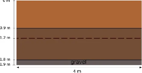
The ASSESS-GPR test site is a cuboid (19 m×4 m×1.9 m) consisting of different well-known sand layers which are uni-form in the short horizontal direction (Buchner et al., 2012). A gravel layer is placed at the bottom 0.1 m to allow for uni-form imbibition and drainage via a pumping tube where the water table height is measured as well. The tube has a diam-eter of 0.47 m and is only perforated over the extend of the gravel. Since the hydraulic conductivity of the gravel can be assumed to be large compared to the one of the sands, the wa-ter is expected to imbibe uniformly over the complete area. In the following we focus on a 4 m long section of the site that consists of two layers plus another compaction horizon formed during the construction of the testbed (Fig. 1).

During the experiment, a stationary GPR antenna was in-stalled at the surface and was set to record a trace every 3 s. We employed a shielded bi-static antenna (Ingegneria dei Sistemi S.p.A., Italy) with a nominal centre frequency of 400 MHz. The transmitter-receiver distance within the an-tenna box is 0.14 m.

[image:2.595.310.546.65.186.2]

Starting at a water table height of 0.47 m, the water ta-ble was altered by imbibing a total amount of 3800 L within 2 h, corresponding to an imbibition rate of 0.0238 m h−1.

Fig. 1. Sketch of geometry of interest shown in vertical cross-section: two different sand layers plus another compaction horizon (dashed line).

Afterwards the system equilibrated for 2 h prior to draining approximately the same amount of water, i.e. 3868 L within 1.5 h (0.0242 m h−1). With the given cross-sectional area of the tank, 80 m2, and by assuming a porosity between 0.3 and 0.4, this led to a maximum amplitude of the water table oscillation of 0.12–0.16 m. GPR traces were recorded during imbibition and drainage and additionally 10–15 min before and after that (Fig. 2).

3 Empirical results

We consider time-series of GPR traces obtained from station-ary antennas and also refer to them as “radargrams”. The in-dividual traces went through minimal postprocessing which consisted of just a dewow filter, which is given as the remain-der of a runmean hat-filter with a width of 5 ns.

3.1 Imbibition

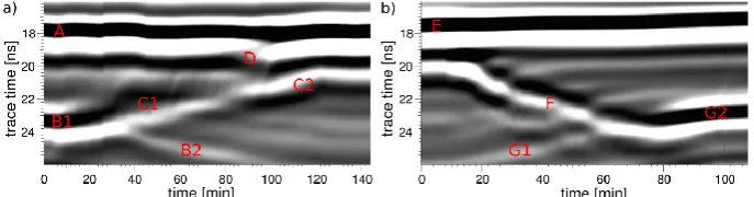
Figure 2a shows an excerpt of the radargram recorded dur-ing the imbibition period, focussdur-ing on travel times between 16 to 26 ns to monitor the dynamics of interest.

We expect reflections from boundaries between different materials and structural differences. We can observe both in the experiment, the latter in the very special case of a compaction. At the beginning (in equilibrium state) there are two sharp reflections, one from the upper layer boundary at 0.90 m depth (A), the other one from the compaction horizon at 1.20 m depth (B1). The reflection wavelets consist of three significant extrema plus a forth weaker one only visible for high intensities.

(3)

[image:3.595.126.470.63.153.2]

Fig. 2. Radargrams recorded during (a) imbibition and (b) drainage. The radargrams show the reflection from the layer boundary at 0.9 m depth (A and E), the reflection from the compaction horizon at 1.2 m depth (B and G) and the capillary fringe reflection (C and F).

static layer boundary would move downwards during the im-bibition, since an increase in water content above the layer boundary is resulting in a lower propagation velocity. Such a behaviour can be observed at (B2) for the reflection from the compaction horizon at 1.2 m depth. In this case one can also observe a phase flip of the wavelet which can be explained by the change of hydraulic properties due to the compaction (Sect. 3.3). At (D) the top of the capillary fringe is reach-ing the upper boundary. The capillary frreach-inge reflection sig-nal gets significantly stronger near the upper boundary (C2) which can be caused either by a sharpening of the capillary fringe due to a capillary barrier at the boundary or by inter-ference with the top layer reflection.

3.2 Drainage

While lowering the water table (Fig. 2b), the shape of the capillary fringe reflection (F) shows the same behaviour as observed in the imbibition period. Due to the variation of the hydraulic conductivity function over several orders of mag-nitude for different water contents in a specific sand, lower water contents translate to a slower relaxation time concern-ing externally induced changes. This means that parts with lower water contents might not be able to follow the water movement, which results in a potential sharpening during im-bibition and widening during drainage. Hence, the shape of the capillary fringe reflection consisting of two extrema can-not be caused by a sharpening of the capillary fringe and the overlying transition zone during imbibition since drainage would show the opposite behaviour and widen the capillary fringe and the transition zone.

The upper boundary reflection is denoted by (E). The cap-illary fringe reflection (F) is well trackable throughout the descent of the water table until the capillary fringe moves through the compaction. After that only the reflection from the lower boundary is visible which is moving upwards dur-ing drainage (G1 to G2). Again the lower boundary reflection shows a phase flip of the wavelet.

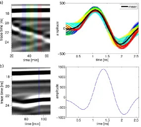
In the following we concentrate on the different shape of the capillary fringe reflection in comparison to an ordinary layer boundary reflection. To retrieve the shape of the cap-illary fringe reflection, we choose the time interval between

32 and 55 min during drainage, where the capillary fringe can be observed without significant interference with the re-flections from the boundaries (Fig. 3a). To illustrate temporal changes and allow for an identification of the characteristic shape, we look at all traces in this time interval, divided into smaller time intervals, marked by differently coloured areas in the radargram. The deformations of the reflection wavelet can be identified as interferences with reflections from struc-tural heterogeneities. As visible in the radargrams, these are frequently present and constantly interfere significantly with the capillary fringe reflection due to its weak amplitude. This emphasises the importance of transient measurements to re-trieve the shape of the capillary fringe reflection. Neverthe-less, the shape of the capillary fringe can be identified as consisting of two extrema. In contrast, the observed reflec-tion from the compacreflec-tion (Fig. 3b) has three significant ex-trema. However, both reflections have a comparable main wavelength.

In the following we will show, with the help of numerical simulations, that the shape of the capillary fringe reflection is closely linked to the general shape of the water retention curve. In fact, this information allows to identify a hydraulic parameterisation most likely describing the water content dy-namics for the observed sand since not every parameterisa-tion is able to reproduce the observed reflecparameterisa-tion.

Before proceeding we complete the recovery of the basic hydraulic dynamics by investigating the observed phase flip of the reflection wavelet from the compaction horizon. 3.3 Impact of the compaction

The observed phase flip of the reflection wavelet can be ex-plained by looking at the change of hydraulic properties due to the compaction.

(4)

[image:4.595.157.443.62.319.2]

Fig. 3. Comparison of reflections from capillary fringe and compaction: (a) capillary fringe reflection taken from the traces marked in the radargram and the resulting mean value. The reflection is sensitive to interference with reflections from heterogeneities, nevertheless a shape with two significant extrema is observable. (b) Reflection from compaction taken out from the trace marked in the radargram. A shape with three significant extrema is observable.

(a) (b)

Fig. 4. (a) Conceptional impact of a compaction on a water retention curve (blue marks the non-compacted, green marks the compacted sand). (b) Exemplary water content distribution for different water tables (blue marks the lower water table) considering a compaction at 0.7 m height.

This has a well-defined impact on the water content dis-tribution around the compaction for different heights of the water table. Figure 4b illustrates this for a sand profile show-ing the discussed properties for two different characteristic water tables with a compaction at 1.2 m depth. The reflection then originates from the jump in water content at the com-paction horizon leading to a jump in the permittivity with the same sign. Following Fresnel’s equation

R = √

ε2− √

ε1 √

ε2+√ε1 (1)

for an incident signal perpendicular to the layer boundary and neglecting conductivity, this translates to a phase flip be-tween different signs in the jump.

For a lower water table, the stronger capillary rise in the compacted sand leads to a higher water content at the com-paction horizon compared to the upper sand. For reasonably higher water tables only the saturated water content deter-mines the jump in water content and thus permittivity at the compaction horizon. Since the permittivity is higher in the upper sand due to the higher water content, one gets a jump in permittivity with an opposite sign, resulting in the observed phase flip.

4 Hydraulic parameterisations

[image:4.595.62.277.393.532.2]

(5)

shape of the capillary fringe reflection, we study the three commonly used hydraulic parameterisations, namely the van Genuchten parameterisation, its simplified version and the Brooks–Corey parameterisation.

The full van Genuchten parameterisation (van Genuchten, 1980) is given by

θ (h)=θr+(θs−θr)1+(αh)n −m

(2) with scale parameterαand shape parametersn,m.

By fixingm= 1−1

n this is simplified to θ (h)=θr+(θs−θr)1+(αh)n−1+

1

n_, ₍₃₎

which is the most commonly used parameterisation in soil hydrology.

Furthermore the Brooks–Corey parameterisation (Brooks, 1966) is given by

θ (h)= (_θ

s h≤ h0

θr+(θs−θr)_hh 0

−λ

h > h0 (4)

with scale parameterh0and shape parameterλ.

5 Numerical simulation

Since the observed behaviour of the capillary fringe reflec-tion is similar for both imbibireflec-tion and drainage, an investiga-tion of the stainvestiga-tionary water content is sufficient.

All stationary water content profiles are calculated using θs= 0.35 andθr= 0.05. This decision represents typical val-ues rather than an optimal estimate, which is also not the intention of this study. The given values just lie in a realis-tic range for a sand. Furthermore a 2 m 1-D sand profile is assumed with a water table at 0.6 m in all cases.

As an input for the GPR simulation, a water content profile is converted to a permittivity profile via the CRIM formula √

ε =θ√εwater+(θs −θ )√εair+(1−θs)√εmatrix (5) usingεair= 1,εwater= 80 andεmatrix= 5.

Since the focus of this study lies on the shape of the re-flection signal and dispersive effects can be neglected in the frequency range used, electric conductivity is set to zero. In-troducing it would only change the total amplitude and not affect the analysis.

We used the FDTD solver Meep (described in Os-kooi et al., 2010). All simulations are carried out in a 2 m×2 m×2.7 m domain including a 0.5 m PML (perfectly matched layer) at each boundary. Forz≤2 m the permittiv-ity is given by the calculated profiles, forz >2 m, above the sand, the permittivity is set toε= 1 for air. The permittivity is assumed to be constant in each horizontal direction.

The transmitter antenna is represented by a point source transmitting a Ricker wavelet with a centre frequency of

f= 400 MHz, polarised inEy-direction. It should be noted that this is not exactly the same source wavelet as observed in the experiment but sufficient to reproduce the observed behaviour. The field inEy-direction is observed over time in 0.2 m distance to represent the receiver antenna. Both points are located 0.02 m above the ground to avoid non physical coupling due to the finite transition width between sand and air coming from the averaging procedure of the permittivity by the algorithm. The spatial discretisation is set to 5 mm to guarantee a good resolution of the capillary fringe and min-imise numerical dispersion.

We now look at the characteristic reflections which can be observed in the modelled data when using the different parameterisations. A special focus is placed on the ability to reproduce the characteristics of the experimental data.

To allow a deeper understanding of the presented re-sults, the general formation of a reflection from a continu-ous permittivity profile is described as conceptualised by the authors.

5.1 Formation of a reflection from a continuous permittivity profile

A given permittivity profile can be described as a compo-sition of infinitesimal thin layers. The reflection signal then results from an infinite number of reflections and transitions originating from the layer boundaries.

Using the linearity of Maxwell’s equations, it is possible to express the incoming wavelet as a superposition of cir-cular monochromatic waves. Depending on the scale of the wave given by the wavelength, the wave is reflected differ-ently from a given feature of the profile.

A wave with a small wavelength compared to the extent of a continuous feature will not be reflected since partial re-flections interfere destructively. A wave with a much longer wavelength on the other hand will experience this feature as a highly localised one and will be reflected accordingly. With this understanding we investigate and explain the character-istic reflections from permittivity profiles calculated with the different hydraulic parameterisations.

5.2 Simplified van Genuchten parameterisation

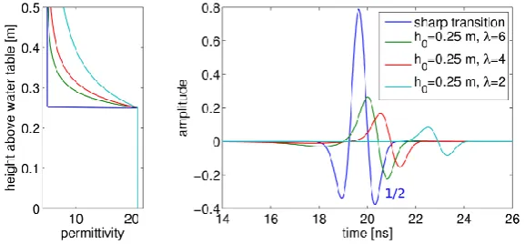
In Fig. 5 we show the different permittivity profiles (right panel) and their resulting modelled reflection signals (left panel). For comparison also a sharp transition is shown (blue).

(6)

[image:6.595.156.442.61.195.2]

Fig. 5. Simplified van Genuchten parameterisation (Eq. 3): permittivity profiles (left panel) and corresponding modelled reflections (right panel) with amplification factor if used. Starting from a realistic set of parameters (green), the impact ofnis shown compared to a sharp transition (blue), while the cyan curve shows an unrealistic parameter set reproducing the measured signal.

Fig. 6. Brooks–Corey parameterisation (Eq. 4): permittivity profiles (left panel) and corresponding modelled reflections (right panel) with amplification factor if used.λis changed while keepingh0constant compared to a sharp transition (blue).

reflection compared to a reflection from a sharp transition are obvious: the main wavelength significantly increases and the signal has a much weaker amplitude. This is caused by the fact that only the low frequency components of the wavelet get reflected due to the width of the transition zone. By in-creasingn (red), the transition zone gets sharpened, corre-sponding to a more localised feature and therefore resulting in an increased amplitude and a smaller main wavelength since also higher frequency components get reflected. Never-theless, the reflected wavelet always consists of three signif-icant extrema, whereas the experiment only shows two sig-nificant extrema.

Only for the very special case of α≥15 m−1 and n of around 2 (cyan), the observed signal shape consisting of only two extrema can be reproduced. However, these parameters do not represent a realistic sand sinceαindicates very large pores, whereas n is more representative for a rather fine-textured material.

Summarizing the results, the simplified van Genuchten pa-rameterisation is not suitable for reproducing the given ex-perimental data and would lead to an erroneous result in a parameter estimation using this parameterisation and capil-lary fringe reflection data.

5.3 Brooks–Corey parameterisation

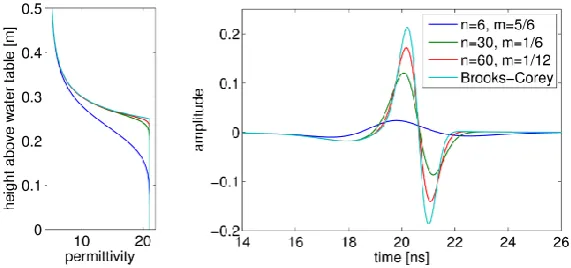
[image:6.595.153.442.252.386.2]

(7)

[image:7.595.154.440.62.196.2]

Fig. 7. Full van Genuchten parameterisation (Eq. 2): permittivity profiles (left panel) and corresponding modelled reflections (right panel). Starting from parameters equal to the simplified van Genuchten parameterisation withα= 4 m−1 andn= 6 (blue),n is increased while n×m= const to sharpen the curve around the air entry. Furthermore, a profile parameterised by the Brooks–Corey parameterisation with h0=1α andλ=n×m(cyan) is shown for comparison.

Comparing the results with Fig. 3, the modelled reflections match the experimental data showing two extrema. Going back to the radargrams (Fig. 2), these extrema correspond to the later part of a reflection from a layer boundary as seen in (C1), for example, when the capillary fringe reflection is separating from the layer boundary reflection.

This shows that reflections from sands parameterised by the Brooks–Corey approach reproduce the characteristic sig-nal changes observed in the experimental data. To emphasise the fact that the different characteristic reflection compared to the simplified van Genuchten parameterisation is a direct consequence of the sharp air entry point, we investigate the full van Genuchten parameterisation. It enables us to con-trol the sharpness around the air entry point by an additional parameter.

5.4 Full van Genuchten parameterisation

In addition toαandn, the full van Genuchten parameterisa-tion includes a second shape parameterm. By settingn×m constant and increasingn, the sharpness at the air entry point can be increased without changing the behaviour for large heights. This is done forα= 4 andn×m= 5, starting with n= 6 (simplified van Genuchten, blue) (Fig. 7).

As the curvature at the air entry point gets sharpened in the permittivity profile (green and red), the shape of the re-flection changes accordingly. The later part of the reflec-tion wavelet gets stronger while the main wavelength de-creases and becomes comparable to the source wavelet. The full van Genuchten parameterisation approaches the Brooks– Corey parameterisation for n→ ∞, λ=n×m and h0=1_α. Still, there remains a difference between the two at a value ofn= 60.

This shows that for a large value ofncompared ton×m, the full van Genuchten parameterisation also reproduces the observed reflection behaviour of the experimental data with two significant extrema. Furthermore, it can be stated that

the key feature in reproducing the observed reflection is the sharpness around the air entry point. Additionally, the ampli-tude is very sensitive to even slight changes in this sharpness. Although we are not able to make a quantitative statement this last point gives a hint to the limitations of the method. The reflection amplitudes in Fig. 7 suggest a high probabil-ity that a sand following the van Genuchten parameterisation with a continuous transition around the air entry might not have a satisfactory signal-to-noise ratio due to the small am-plitudes of the reflection. This fact also gives the limitations concerning a quantitative estimation of hydraulic parame-ters. In all cases the reflection originating from the transition above the air entry has a very small amplitude, presumably in the range of the deviations over time shown in Fig. 3b.

6 Conclusions

It was shown that an on-ground 400 MHz GPR system can provide valuable information about the basic shape of the capillary fringe without any further complex post-processing. Simulations show that this can be used to select an appropriate hydraulic parameterisation for the observed sand which is an essential but often neglected aspect of esti-mating hydraulic properties. This is possible since the differ-ent commonly used parameterisations discussed here show significantly different reflections.

While the simplified van Genuchten parameterisation with m= 1−1

(8)

Nevertheless, the amplitude can vary significantly with a slight change of this sharpness by the full van Genuchten parameterisation.

Acknowledgements. This work was funded in part by Deutsche

Forschungsgemeinschaft (DFG) through project RO 1080/8-2. The simulations where carried out at the servers of bwGRiD (http://www.bw-grid.de), member of the German D-Grid initiative, funded by the Ministry for Education and Research (Bundesminis-terium für Bildung und Forschung) and the Ministry for Science, Research and Arts Baden-Wuerttemberg (Ministerium für Wis-senschaft, Forschung und Kunst Baden-Württemberg). We would also like to thank all the members of our group helping to carry out the described experiment.

Edited by: N. Romano

References

Brooks, R.: Properties of porous media affecting fluid flow, J. Irrig. Drain. Div.-ASCE, 92, 61–88, 1966.

Buchner, J. S., Wollschl¨ager, U., and Roth, K.: Inverting surface GPR data using FDTD simulation and automatic detection of reflections to estimate subsurface water content and geometry, Geophysics, 77, 1–11, doi:10.1190/GEO2011-0467.1, 2012. Endres, A., Clement, W., and Rudolph, D.: Ground penetrating

radar imaging of an aquifer during a pumping test, Ground Wa-ter, 38, 566–576, 2000.

Iden, S., Durner, W., and Schelle, H.: Combined transient method for determining soil hydraulic properties in a wide pressure head range, Soil Sci. Soc. Am. J., 75, 1681–1693, 2011.

Ippisch, O., Vogel, H., and Bastian, P.: Validity limits for the van Genuchten-Mualem model and implications for parameter esti-mation and numerical simulation, Adv. Water Resour., 29, 1780– 1789, 2006.

Lambot, S., Rhebergen, J., Van den Bosch, I., Slob, E., and Van-clooster, M.: Measuring the soil water content profile of a sandy soil with an off-ground monostatic ground penetrating radar, Va-dose Zone J., 3, 1063–1071, 2004a.

Lambot, S., Slob, E. C., van den Bosch, I., Stockbroeckx, B., Scheers, B., and Vanclooster, M.: Estimating soil electric prop-erties from monostatic ground-penetrating radar signal inver-sion in the frequency domain, Water Resour. Res., 40, W04205, doi:10.1029/2003WR002095, 2004b.

of unsaturated porous media, Water Resour. Res., 12, 513–522, 1976.

Oskooi, A. F., Roundy, D., Ibanescu, M., Bermel, P., Joannopou-los, J., and Johnson, S. G.: Meep: a flexible free-software pack-age for electromagnetic simulations by the FDTD method, Com-put. Phys. Commun., 181, 687–702, 2010.

Russo, D.: Determining soil hydraulic properties by parameter esti-mation: on the selection of a model for the hydraulic properties, Water Resour. Res., 24, 453–459, 1988.

Saintenoy, A., Schneider, S., and Tucholka, P.: Evaluating ground penetrating radar use for water infiltration monitoring, Vadose Zone J., 7, 208–214, 2008.

Schindler, U., von Unold, G., Durner, W., and M¨uller, L.: Evapo-ration method for measuring unsaturated hydraulic properties of soils: extending the measurement range, Soil Sci. Soc. Am. J., 74, 1071–1083, 2010.

Simunek, J., van Genuchten, M., Gribb, M., and Hopmans, J.: Pa-rameter estimation of unsaturated soil hydraulic properties from transient flow processes, Soil Till. Res., 47, 27–36, 1998a. Simunek, J., van Genuchten, M., and Wendroth, O.: Parameter

es-timation analysis of the evaporation method for determining soil hydraulic properties, Soil Sci. Soc. Am. J., 62, 894–905, 1998b. Steelman, C. and Endres, A.: Assessing vertical soil moisture

dy-namics using multi-frequency GPR common-midpoint sound-ings, J. Hydrol., 436–437, 51–66, 2012.

Tsoflias, G., Halihan, T., and Sharp Jr., J.: Monitoring pumping test response in a fractured aquifer using ground-penetrating radar, Water Resour. Res., 37, 1221–1229, 2001.

Van Dam, J., Stricker, J., and Droogers, P.: Inverse method to de-termine soil hydraulic functions from multistep outflow experi-ments, Soil Sci. Soc. Am. J., 58, 647–652, 1994.

van der Kruk, J., Jacob, R. W., and Vereecken, H.: Properties of precipitation-induced multilayer surface waveguides derived from inversion of dispersive TE and TM GPR data, Geophysics, 75, 263–273, doi:10.1190/1.3467444, 2010.

van Genuchten, M.: A closed-form equation for predicting the hy-draulic conductivity of unsaturated soils, Soil Sci. Soc. Am. J., 44, 892–898, 1980.

Vereecken, H., Kaiser, R., Dust, M., and P¨utz, T.: Evaluation of the multistep outflow method for the determination of unsaturated hydraulic properties of soils, Soil Sci., 162, 618–631, 1997. Wollschl¨ager, U., Pfaff, T., and Roth, K.: Field-scale apparent