Abstract---The main objective of Automatic Generation Control (AGC) is to maintain balance between the total system generations against system load fluctuations, maintaining scheduled frequency and net power interchange with neigh boring areas in an interconnected power system. Any mismatch between generation and demand causes deviation in frequency, where high deviation in frequency may lead to system collapse. Thus the system frequency should be controlled. This paper deals with the tuning of AGC of a two area interconnected thermal system using P-I-D controllers. Parameters of these controllers are derived using Many Optimizing Liaisons (MOL) Technique. Dynamic Response and Robustness of the PID controlled AGC, tuned by both the techniques are compared applying 1% step load perturbation in both areas at different conditions. The results reported in this paper demonstrate the effectiveness of MOL over PSO in the tuning of AGC parameters.
Index Terms---Automatic Generation Control, Area Control Error, Many Optimizing Liaisons algorithm, Proportional-Integral-Derivative controller.
I. INTRODUCTION
In an interconnected Power System, the control areas are to be interconnected in order to generate, transport and distribute electric energy maintaining a constant frequency and terminal voltage under normal as well as under load fluctuations. However the imbalance between the generated and consumed power, results in change in nominal frequency . When the amount of the generated power is more than the amount of power demand, then the frequency of the system increases and vice versa. In order to maintain the frequency and the tie line power flow at their scheduled value automatic generation control (AGC) is used.
The first attempt in the area of AGC has been to control the frequency of a power system via the governor of the synchronous machine. This technique was subsequently found to be insufficient and a supplementary control was included to the governor with the help of a signal directly proportional to the frequency deviation plus it‟s integral. The system nominal frequency depends on balance between the real powers generated and consumed. Cohn has initiated early works on AGC[2].Lee and Coworkers in1991,proposed the first self tuning control method for AGC[3].Talaq suggested a fuzzy gain scheduling method for conventional PI controller in [4]. P V Pradeep Reddy1, M.Tech, Department of EEE , Sri Venkateswara University College of Engg ,Sri Venkateswara University
Titupati,India.
V.Usha Reddy2 ,Asst.Prof.Dept.of EEE, Sri Venkateswara University College of Engg,Sri Venkateswara University, Tirupati,India.
Gozde and Taplamacioglu, proposed PSO algorithm for AGC system for an inter connected thermal power plants in 2011[5].Almost all past works were to be appreciated that the overall performance of AGC in any power system depends on the proper design of both primary control loop i.e. selection of R and secondary control loops i.e. selection of gain for supplementary controller. Over the past decades, many control strategies have been proposed for AGC viz. Proportional and integral (PI), Proportional, Integral and Derivative (PID) and Optimal controllers.
M.E.H.Pedersen,A.J.Chipperfield[10],proposed Simplifying particle swarm optimization using[8,9] in the year 2009.
B.K Sahu and P.K. Mohanty [6,7] have discussed the modeling and comparative analysis of PID controller of Automatic Voltage Control system via Many Optimizing Liaisons.
The main features of AGC loops are to maintain i. Frequency at scheduled value.
ii.Net interchanges of power with neighboring areas. In this paper, PID controllers are used to improve the dynamic performance of AGC of a two area thermal system.
Proportional Integral Derivate (PID) controller
The PID controller has been successfully used for over 50years. It is a robust, easily understood controller that can provide excellent control performance despite the varied dynamic characteristics of control areas. PID controller consists of three basic modes, the proportional mode, the integral and the derivative modes. A proportional controller has the effect of reducing the rise time, but never eliminates the steady-state error. If the proportional gain is too high ,the system can become unstable where as a small gain results in a small output response to a large input error, and a less responsive or less sensitive controller. An integral controller has the effect of eliminating the steady-state error, but it may obtain weak transient response. High integral gain can cause overshoot and low value will make the system sluggish. A derivative controller has the effect of increasing the stability of the system, reducing the overshoot, and improving the transient response. If the derivative gain is sufficiently large it can cause a process to become unstable. The gains of the controller are tuned by the MOL.
The main aim of this work is the application of MOL algorithm to tune the parameters of the PID controllers in an interconnected system. In view of the above, the present work investigates the following aspects:
i)To optimize the parameters of the conventional PID controllers using MOL algorithm.
Many Optimizing Liaisons based Assessment of
PID Controller Performance for Automatic
Generation Control
ii) To compare the performance of MOL optimized PID controlled AGC for two area interconnected thermal power system with [1].
II. PROPOSED METHOD
In order to represent a basic simple model of an interconnected power system, in this work deal with two Thermal areas of equal size of 1000MW consisting both reheat with governor dead band mechanism. The introduction of dead band makes the system non-linear.
Fig.1 Block diagram of two area interconnected Thermal system In the design of PID controllers (two in number) for this work the six gains are selected in such a way that the desired response obtained of the closed loop system which refers that the system should have a minimum settling time and a very less value of overshoot as well as undershoots with less oscillations due to a 1% Step Load Perturbation as
1
1 1 1 1 1 1 ACE dt d K dt ACE K ACE K u p i
d (1)
2
2 2 2 2 2 2 ACE dt d K dt ACE K ACE K u p i
d (2) The value of Area Control Error is sum of bias factor and tie-line power deviation. The area control error in both areas consists of tie-line power error of the intermediate area and frequency error, given by𝐴𝐶𝐸1 = 𝐵1 + Δ𝑃𝑇𝐼E (3)
𝐴𝐶𝐸2 = 𝐵2 + Δ𝑃𝑇𝐼𝐸 (4)
In this work, the constraint of setting the gains of PID controller is a major problem. Therefore, the PID gains should be in limits, i.e.,
Kpmin ≤ Kpi ≤ Kpmax Kimin ≤ Kii ≤ Kimax Kdmin ≤ Kdi ≤ Kdmax
Where i is the number of controller gains (here i = 2 due to two controllers).
𝐾𝑝, and 𝐾𝑑𝑚𝑖𝑛 are the minimum values of controller parameters and maximum allowable values of controller parameters are 𝐾𝑝𝑚𝑎x, 𝐾𝑖𝑚𝑎𝑥 and 𝐾𝑑𝑚𝑎𝑥
Hence forth, in this work PID parameters are constrained with in [0, 2.5].
The main aim of tuning the system is minimizing the value of Area Control Error (ACE). In order to achieve this, the fitness function J is taken as
𝐽 = (5) Where ACEi= Area control error of ith area,
T = simulation time.
III. Tuning algorithm used in the proposed work Many Optimizing Liaisons Algorithm
In this paper the response of simplified PSO algorithm named Many Optimizing Liaisons (MOL) which was proposed by Pedersen and Chipper field in 2009[10] has been evaluated, to derive the PID controller parameters by minimizing the error, coordinated with the frequency control. By setting the parameter C1 = 0, MOL removes the need for an
extra random deviate in velocity recurrence relation and most importantly, eliminates the need for a previous best solution for every particle. Instead of iterating over all agents in the swarm as done normally in PSO [1], the MOL picks the agent to update at random, thereby minimizing the memory and time used for computation.
The MOL algorithm. Step 1:
Initialize the values of time constants of governor „Tg‟,reheat „Tr‟,turbine „Tt‟ and power system „Tp‟.in their respective control areas.
Initialize the values of Kp, R1,R2,and primary control loop gains B1 and B2 in their respective control areas.
Step 2
Initialization of particles
Initialize xi where i= 1…....n with D uniform random values
each representing the gains of PID controller with upper and lower bounds „0.1‟ and „2.5‟ respectively.
Here Dimension is taken for particles as [1x6]. Step 3
Initialization of random vector
Random variables are chosen within limits i.e.; rand U[0, 1)
Step4
Initialization of vector g
Initialize vector g with random locations in all D dimensions. Evaluate the fitness of vector g using best of particles, pbest.
Calculate the fitness of vector
x
i , for which ACE=0(3&4). Step 5Update the Velocity of particles
)
(
2
2
)
(
1
1
) 1 ( t i i t i i t i ti
w
V
C
rand
pbest
P
C
rand
gbest
P
V
By making the parameter C1=0, eliminates particle best, there by equation is rewritten as 2
(
)
) 1 ( t i i t i t iV
C
rand
gbest
x
V
(6) Step 6Update the position of Particles
Using below equation the position of particle is updated
) 1 ( ) 1 (
t i t i t ix
V
X
(7) Step7
The above steps are repeated for swarm‟s best Position f (gbest) which represent the best controller gains in minimizing Area Control Error.
IV. RESULTS AND DISCUSSION
The AGC system with PID controllers tuned by MOL algorithm is shown in fig 1.The gains of the PID controllers are tuned by MOL algorithm. If proportional gain (kp) is very
high the system can become unstable where as a small gain results in a small output response to a large input error, and a less responsive or less sensitive controller. High integral gain (Ki) can cause overshoot and low value will make the system
sluggish. If the derivatives gain (kd) is sufficiently large it can
cause a process to become unstable. These gains depend on the process to be controlled. For an AGC system the typical ranges used in literature are (0.1-2.5).After running the optimization algorithm for several times it is found that the minimum and maximum values of gains for different objective functions lie in the chosen range. A small step load perturbation (SLP) of 1% is applied to both areas to study the dynamic response of the PID controlled AGC. The optimum values of PID controller gains are depicted in table I.
TABLE I
Optimum gains of PID for both areas tuned by PSO and MOL algorithm
Algorithm PID controller gains for PID controller gains for
area-1 area-2
Parameters Kp1 Ki1 Kd1 Kp2 Ki2 Kd2
PSO 2.3285 2.4883 1.5280 1.7152 1.1256 1.8945
MOL 1.1112 1.8311 1.4328 1.4251 2.2472 2.2194
The settling time and peak overshoots of ΔF1 ,ΔF2 and
ΔPtie are tabulated below employing PSO[1] and MOL algorithms.
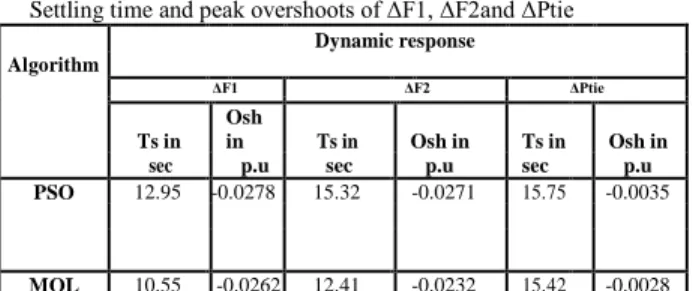
TABLE II
Settling time and peak overshoots of ΔF1, ΔF2and ΔPtie
Dynamic response Algorithm ΔF1 ΔF2 ΔPtie Ts in Osh in Ts in Osh in Ts in Osh in
sec p.u sec p.u sec p.u
PSO 12.95 -0.0278 15.32 -0.0271 15.75 -0.0035
MOL 10.55 -0.0262 12.41 -0.0232 15.42 -0.0028
From table I and table II it is clearly shown that the dynamic response i.e. change in frequency and change in tie line power is optimized employing MOL technique.
From fig.2, fig.3 andfig.4 respectively shows the variations in ΔF1,ΔF2 and ΔPtie for both PSO [1] and MOL algorithms and thus concludes that MOL has better transient behavior over algorithm employed in[1].
Time in seconds (30)
Figure 2 Frequency deviation in area-1 F re q u en cy d ev ia tio n in a re a -1 (H z) F re q u en cy d ev iati o n in a re a-2 (Hz )
Time in seconds (30)
Figure 3 Frequency deviation in area-2
Time in seconds (30) Figure 4 Tie Line power deviation
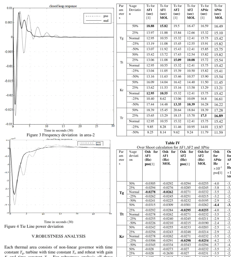
V.ROBUSTNESS ANALYSIS
Each thermal area consists of non-linear governor with time constant Tg, turbine with time constant Tt, and reheat with gain Kr and time constant Tr . For robustness analysis all these
parameters are varied from -50% to +50% in steps of 25% by applying 1% SLP in both areas. The controller gains obtained from [1] and MOL algorithm are used and compared to study the robustness of the system.
Table III
Settling times Ts for ΔF1,ΔF2 and ΔPtie
Par am eter s %age Deviatio n Ts for ΔF1 (sec) [1] Ts for ΔF1 (sec) MOL Ts for ΔF2 (sec) [1] Ts for ΔF2 (sec) MOL Ts for ΔPtie (sec) [1] Ts for ΔPtie (sec) MOL Tg 50% 18.88 15.82 19.5 16.47 16.59 16.49 25% 13.97 11.88 15.84 12.66 15.32 15.10 Normal 12.95 10.55 15.32 12.41 15.75 15.42 -25% 13.19 11.08 15.45 12.55 15.91 15.82 -50% 13.07 11.92 15.43 12.41 15.85 15.75 Tt 50% 15.42 13.72 17.43 12.54 15.82 15.82 25% 13.06 11.08 15.09 10.08 15.72 15.54 Normal 12.95 10.55 15.32 12.41 15.75 15.42 -25% 13.04 11.05 15.39 10.50 15.82 15.41 -50% 13.16 11.63 15.46 10.57 15.90 15.54 Kr 50% 16.09 14.04 16.42 14.40 11.50 11.45 25% 13.62 11.53 15.16 13.58 13.29 13.21 Normal 12.95 10.55 15.32 12.41 15.75 15.42 -25% 10.40 8.62 13.06 10.09 16.8 16.61 -50% 17.44 14.48 13.35 10.39 16.28 16.22 Tr 50% 18.39 15.45 20.64 18.84 18.39 17.28 25% 15.65 13.29 18.15 15.70 17.5 16.89 Normal 12.95 10.55 15.32 12.41 15.75 15.42 -25% 9.85 8.28 11.46 10.95 14.01 13.97 -50% 8.25 8.14 9.62 9.24 11.79 11.59 Table IV
Over Shoot calculation for ΔF1,ΔF2 and ΔPtie
Par am eter s %age deviati on Osh for ΔF1 (Hz) pso[1] Osh for ΔF1 (Hz) MOL Osh for ΔF2 (Hz) pso[1] Osh for ΔF2 (Hz) MOL Osh for ΔPtie Hz 3 10 pso[1] Osh for ΔPti e Hz 3 10 MOL Tg 50% -0.0305 -0.0292 -0.0294 -0.0255 -4.0 -3.3 25% -0.0294 -0.0276 -0.0285 -0.0245 -3.8 -3.1 Normal -0.0278 -0.0262 -0.0271 -0.0232 -3.5 -2.8 -25% -0.0262 -0.0245 -0.0251 -0.0215 -3.2 -2.6 -50% -0.0241 -0.0225 -0.0232 -0.0195 -2.9 -2.5 Tt 50% -0.0315 -0.0309 -0.0301 -0.0262 -4.4 -3.6 25% -0.0292 -0.0284 -0.0295 -0.0255 -4.0 -3.3 Normal -0.0278 -0.0262 -0.0271 -0.0232 -3.5 -2.8 -25% -0.0255 -0.0240 -0.0245 -0.0211 -2.9 -2.4 -50% -0.0226 -0.0210 -0.0215 -0.0190 -2.4 -2.1 Kr 50% -0.0242 -0.0255 -0.0233 -0.0203 -2.5 -1.9 25% -0.0256 -0.0243 -0.0248 -0.0214 -2.9 -2.3 Normal -0.0278 -0.0262 -0.0271 -0.0232 -3.5 -2.8 -25% -0.0306 -0.0291 -0.0298 -0.0254 -4.2 -3.6 -50% -0.0345 -0.0334 -0.0343 -0.0294 -5.7 -4.9 Tr 50% -0.028 -0.0273 -0.027 -0.0232 -3.5 -2.9 25% -0.028 -0.2630 -0.027 -0.0231 -3.5 -2.8 Normal -0.027 -0.0262 -0.0271 -0.0232 -3.5 -2.8 -25% -0.0278 -0.0260 -0.0270 -0.0229 -3.5 -3.4 -50% -0.0276 -0.0261 -0.0628 -0.0230 -3.4 -2.7
Table III and IV shows the transient behavior of interconnected power system optimization using reference[1] and MOL algorithm.
From the tables the robustness analysis gives the idea of controlled operation of particular respective tuned PID gain
F re q u en cy d ev ia tio n in Ti el in e (H z )
values with a 1% step disturbance on both areas and we can restore the system into a new operating point with minimum deviation in ACE.
VI. CONCLUSION
The results obtained from the simulation studies show that the MOL tuned system achieves better dynamic performance, i.e., less Overshoot, better settling times than the results obtained in [1] . From the study it can be concluded that PID controlled AGC for the two area interconnected system tuned by MOL algorithm gives acceptable and reliable management the frequency and tie line power deviations(ΔPtie).There by it can be concluded as Many Optimizing Liaisons gives comparatively better and faster performance over PSO algorithm[1]. APPENDIX Tg1=Tg2=0.3s,Tt1=Tt2=0.8s, Tp=20s,Tr=10sT12=0.707 B1=B2=0.425p.u.MW
/
Hz, Kr=0.5, Kp=120Hz/
p.u., R1=R2=2.4Hz/
p.u, REFERENCES[1] B.K.Sahu, Itishree Ghatuari, N.Mishra.“Performance analysis of AGC of a two area interconnected thermal system with non-linear governor using PSO and DE algorithm.” 978-1-4673-6150-7/13/ ©2013 IEEE.
[2] Cohn N. “Some aspects of tie-line bias control on interconnected power systems”. An Inst Elect Eng Trans 75 (1957) 1415–36.
[3] Lee KA,Yee H,teo CY .“Self-tuning algorithm for automatic generation control in an interconnected power system.”Elect Power Syst Res 20(2) (1991)157-65.
[4] Talaq J,Al-Basari F .“Adaptive fuzzy gain scheduling for Load frequency control”.IEEE Trans Power systems 14(1)(1999) 145-50.
[5] H.Gozde,M.C.Taplamacioglu.“Automatic Generation Control Application with craziness based particle swarm optimization in a thermal power system.” Electrical power and Energy systems 33(2011)8-16.
[6] B. K. Sahu, P. K. Mohanty. “Design and Comparative Performance Analysis of PID Controlled Automatic Voltage Regulator tuned by Many Optimizing Liaisons.” 978‐1‐4673‐2043‐6/12/ ©2012 IEEE.
[7] B K Sahu, P K Mohanti. “Design and performance analysis of PID controller for AVR using Simplified particle Swarm Optimization.” ELSEVIER June 2012.
[8] Kennedy J, Eberhart R. “Particle Swarm Optimization.” . Perth,Australia: IEEE International Conference on Neural Networks, 1995.
[9] Shi, Y, Eberhart, R. “ A Modified Particle Swarm Optimizer.” Anchorage, AK, USA: IEEE International Conference on Evolutionary Computation, 1998.
[10] M.E.H. Pedersen, A.J. Chipper field, “Simplifying particle swarm optimization.” Applied Soft Computing 10 (2010) 618–628.
About Authors:
P.V.Pradeep Reddy1 is presently pursuing
M.Tech in Department of Electrical Engineering,
Sri Venkateswara University College of
Engineering, Tirupati, India. He received his
B.Tech degree from Jawaharlal Nehru
Technological University, Anantapur in the year 2012. His areas of interest include electrical power systems, nuclear engineering,electrical machines and renewable energy resources.
V. Usha Reddy2 has submitted her Ph.D in Jawaharlal Nehru Technological University College of Engineering, Hyderabad, India. She received her M.Tech from Sri Venkateswara University College of Engineering, Tirupati, India in 2007 and B.Tech from Jawaharlal Nehru Technological University, Hyderabad, India in 2003. Currently she is working as Assistant Professor in Department of Electrical Engineering, Sri Venkateswara University College of Engineering, Tirupati, India from last 7 years. She has 24 international journals, 5 international conferences publications. She has guided 10 M.Tech projects. Her specialization is Power Systems Operation and Control.