Bounds Testing Approach to Analyzing the Environment Kuznets Curve Hypothesis: The Role of Biomass Energy Consumption in the United States with Structural Breaks

(1)

Munich Personal RePEc Archive

Bounds Testing Approach to Analyzing

the Environment Kuznets Curve

Hypothesis: The Role of Biomass Energy

Consumption in the United States with

Structural Breaks

Shahbaz, Muhammad and Solarin, Sakiru Adebola and

Hammoudeh, Shawkat and Shahzad, Syed Jawad Hussain

Montpellier Business School, Montpellier, France, Multimedia

University Malaysia, Melaka, Malaysia, Lebow College of Business,

Drexel University, United States

3 October 2017

Online at

https://mpra.ub.uni-muenchen.de/81840/

(2)

1 Bounds Testing Approach to Analyzing the Environment Kuznets Curve Hypothesis:

The Role of Biomass Energy Consumption in the United States with Structural Breaks

Muhammad Shahbaz

Montpellier Business School, Montpellier, France Email: [email protected]

Sakiru Adebola Solarin

Faculty of Business and Law

Multimedia University Malaysia, Melaka, Malaysia Email: [email protected], Phone: +6042523025

Shawkat Hammoudeh*

Lebow College of Business, Drexel University, United States Energy and Sustainable Development,

Montpellier Business School, Montpellier, France Email: [email protected]

Syed Jawad Hussain Shahzad

COMSATS Institute of Information Technology, Islamabad Pakistan & University of Malaysia Terengganu, Malaysia

E-mail: [email protected]

Abstract: This paper re-examines the specification of the environmental Kuznets curve (EKC)

for the US economy by accounting for the presence of a major renewable energy source and trade openness over the period 1960-2016. Biomass energy consumption and trade openness as well as oil prices are considered as additional determinants of economic growth, and consequentially of CO2 emissions. The bounds testing approach to cointegration is applied to

examine the long-run relationship between the variables in the presence of structural breaks. The causal relationship between the variables is investigated by applying the VECM Granger causality test by accommodating structural breaks. The results confirm the presence of cointegration between the variables. Moreover, the relationship between economic growth and CO2 emissions is not only inverted-U shaped but also N-shaped in the presence of structural

breaks and biomass. Biomass energy consumption lowers CO2 emissions. Exports, imports and

trade openness are also environment- friendly. The causality analysis indicates a feedback effect between biomass energy consumption and CO2 emissions. Economic growth still Granger causes

CO2 emissions in this new setup.

Keywords: EKC; Biomass energy; Oil prices; Trade openness; Structural breaks.

(3)

2

1. Introduction

The environment has attracted unprecedented attention from ecologists, researchers and policymakers in recent years. While the objective of the diverse stakeholders is to maintain a high living standard and reduce global poverty, which can be considered justifiable ends in their own right, an unrestricted exploitation of natural resources could also cause an irrevocable loss to the biosphere and hurt the world’s long-term economic and social development objectives. The catch lies in the fact that the environment cannot be sustained without sacrificing at least some of long-term growth and development objectives. Consequently, to satisfy some basic human needs, some damage to the environment is inevitable. Attitudes towards the environment vary substantially, particularly among policymakers. Even if the biosphere can be exploited in a variety of ways which lead to a range of consequences, many ecologists believe that the ecosystem could be managed in a way that it can adapt itself to continuously changing conditions (El-Kholy et al. 2012).

The environmental Kuznets curve (EKC), as a theory of the relationship between economic development and environmental quality, hypothesizes that over time that there will be a reduction in the level of emissions for most countries. This reduction can take place possibly because well developed economies should develop and raise sufficient revenues in the long-run to afford newer and cleaner technologies that can help abate pollution. Environmental degradation stands a huge cost in terms of health and life sacrifices. According to recent estimates, outdoor pollution kills more than three million people in the world every year, while many more people suffer from a range of diseases (OECD, 2014).

(4)

3 the increased revenues resulting from higher growth are used to pursue overly redistributive policies (Bhagwati and Panagariya, 2014). However, the existing development paradigm is unsustainable because it favors a level of prosperity, which invariably results in more consumption and greater pressure on natural resources (Aşıcı, 2013).

Sustainable economic growth depends on the availability of renewable energy sources, and the integrated development of such sources is essential for an environmentally friendly development of countries or regions. One of the widely used sources of renewable energy in the United States is biomass which is any organic (decomposable) matter derived from plants or animals, and hence is available on a renewable basis. Biomass includes wood and agricultural crops, herbaceous and woody energy crops and municipal organic wastes as well as manure. This renewable source of energy contains a complex mix of carbon, nitrogen, hydrogen and oxygen. Unlike the conventional fossil fuels such as petroleum and coal, biomass is a source of renewable energy based on the carbon cycle. Thus, in virtue of its abundant sources, biomass is likely to be a prevalent option for generating electricity in the future.

(5)

4 The results find cointegration between carbon emissions and their determinants and highlight that biomass energy consumption improves environmental quality by lowering carbon emissions. Moreover, the relationship between economic growth and carbon emissions is inverted U-shaped (i.e. EKC exists) and N-shaped in the presence of biomass energy consumption and structural breaks. Additionally, trade openness (exports, imports) is inversely linked with carbon emissions in the presence of biomass energy consumption. The causality analysis demonstrates a feedback effect between biomass energy consumption and carbon emissions, while economic growth causes CO2 emissions. The causal association between trade

openness (exports, imports) and carbon emissions is bidirectional.

The remainder of study is organized as follows. Section-2 surveys the literature on EKC, biomass energy consumption and trade openness. Section-3 develops the empirical model and Section-4 presents the methodological framework. Section-5 discusses the empirical results. Section 6 provides the conclusion and policy implications.

2. Biomass energy consumption and regulations in the U.S.

In comparison with the other sources of energy, biomass provides a distinctive advantage with respect to maintaining the environment since it is “carbon neutral”. Although the combustion of biomass generates as much carbon dioxide as fossil fuels do, CO2 emissions

released is removed when a new plant grows (Agbor et al. 2014; A-Mulali et al. 2016). In other words, some CO2 emissions from one year’s combustion of biomass are captured by future biomass crops through the process of photosynthesis. In relation to its energy uses by industry, biomass energy can be used for heat or power generation or for combined heat and power generation as a direct substitute for fossil fuels. In short, the biomass use is growing in significance as an input to a number of major functions of industries, ranging from research into an application of material inputs to industrial processes through to an implementation of mass produced intermediate and final products (Burritt and Schaltegger, 2012).

(6)

5 increases in biofuel trade are also considered a potential driver of economic growth in the tropics and subtropics regions, which are likely to hold a comparative advantage in feedstock production due to high biomass productivity (Marshall, 2007).

Biomass energy is one of the earliest and most primary sources of energy to provide processing and heat for industrial facilities in the United States. Historically in this country, it has come from three primary sources: wood, waste, and alcohol fuels. More recently, it has come from corn as well. Each of these forms of biomass energy (wood energy, waste energy and biofuel) is used in the United States. Collectively, they represent almost half of the total renewable energy production. Most electricity generation from wood biomass occurs at lumber and paper mills. These facilities use wood waste to provide much of their own steam and electricity needs.

The adoption of biomass has been increasing over the years in the United States. Biofuel production increased from 1,382 ktoe in 1990 to 3,000 ktoe in 2000, and further to 28,440 in 2013 (BP Statistical Review of World Energy, 2014). Over the years, the U.S. government has introduced several policies to improve the share of renewable energy in the total energy mix, including an increase in the use of biomass. For instance, the Renewable Portfolio Standard (RPS) policy, which is a state regulation, calls on electric utilities to ensure that a specific percentage of all produced electricity should come from renewable resources. The first RPS was ratified in Iowa in 1983, under a slightly different name, but with the same basic construction. The 1990s really sparked the adoption of RPS, as seven more U.S. states enacted RPSs of similar varieties. Currently there are 30 states, along with the District of Columbia, that have adopted some form of an RPS policy. RPS allows for ample state flexibility including a variation of different target goals and deadlines, market trading mechanisms and renewable energy types used to comply with the RPS policy. This flexibility makes this particular policy tool especially popular, as evident by the recent exponential increase in RPS adoption. Even though the adoption of RPS is becoming rather common, this policy tool is still relatively new, with few scholarly attempts at ascertaining the results of its implementation (Eastin et al., 2014).

(7)

6 part of the Energy Policy Act in 2005 in an effort to reduce greenhouse gases emissions and expand the nation’s renewable fuels sector, while reducing reliance on imported oil (Barbos et al., 2011). The RFS program was expanded under the Energy Independence and Security Act of 2007. The RFS was conceived by policy makers as a tool to reduce the demand for transportation fuels derived from foreign oil by stimulating the production of domestic biofuels that could be mixed with or replace gasoline at a time when foreign imports and prices were at or near all-time highs. The RFS, administered by the US Environmental Protection Agency (EPA), mandates the annual minimum volumes of biofuels across four nested categories that must be incorporated into the nation’s transportation fuel supply. The biofuel categories include total renewable fuels, advanced renewable fuels, cellulosic biofuel, and biomass-based biodiesel. It also requires electricity providers to acquire specific amounts of renewable energy generation over time which are prevalent within the United States (Barbos et al., 2011).

The government has also introduced several additional policies including the Production Tax Credit or PTC, which is a per-kilowatt-hour tax credit for electricity generated (through renewable energy sources including biomass) by qualified energy resources and is paid for by the U.S. taxpayers. These policies also include the Investment Tax Credit or ITC, which allows the tax credit to be taken based on the amount invested rather than electricity produced. They also include the Modified Accelerated Cost Recovery System Depreciation Schedule or MACRS, which gives bonus depreciations and reduces taxes on large biomass projects (Zhou et al. 2016).

3. Literature review

(8)

7 method of estimation with panel data assumes that all cross-sections adhere to the same EKC, it may be unreasonable to impose isomorphic EKCs if cross-sections vary in terms of resource endowments, infrastructure, etc. (List and Gallet, 1999)1_{. We classify the considered literature}

under three strands: income and emissions; energy consumption and income; and energy consumption, income and carbon emissions.

3.1 Income and emissions

This first strand of the literature has considered income as the only determinant of emissions within the EKC framework in the United States. For instance, Unruh and Moomaw (1998) utilize graphical analysis to examine the presence of EKC for 16 countries including the United States. Using a data set for the period 1950-1990, these authors are able to provide evidence of the presence of EKC in the U.S. Subsequently, List and Gallet (1999) analyze the presence of EKC in the 50 U.S. states by using the ordinary least square (OLS) technique for the period 1929-1994. They confirm the presence of EKC in 18 states when income and income squared are entered as independent variables, with the mono-nitrogen oxides serving as the indicator of emissions. However, when income and income squared are entered as independent variables, and with sulfur dioxide serving as the indicator of emissions, they notice the presence of the N-shaped for 10 states.

3.2 Energy and income

The papers on the causal relationship between energy consumption (or its various components) and real GDP constitute the bulk of the existing literature that uses the bivariate and multivariate approaches. This strand is also the earliest part of the literature dating back to 1978. We will focus on this aspect of the literature because it is believed that energy consumption and real income are associated with emissions. The earliest papers have utilized the bivariate approach to consider the relation between energy consumption and economic growth but provided inconclusive empirical results for the US economy 2_.

1_{In this paper, we concentrate on the time series literature associated with the concept of EKC in the United States.}

In the cases where the study involves a multi-country data set, we only report the results for the United States.

2_{For example, Kraft and Kraft (1978), Akarca and Long (1979), Erol and Yu (1987a, b), Yu et al. (1988), Lee}

(9)

8 The earliest studies that also looked at the relationship from a multivariate perspective including Glasure and Lee (1995) which added the ratio of wages and energy prices as control variables for the period 1973:M1-1984:M6. Using the Engle and Granger (1987) method, their

findings provide evidence that supports the neutrality hypothesis. Similarly, Stern (2000) employs the Johansen (1988) and Johansen and Juselius (1990) to examine the relationship between energy use, capital, labor and real GDP for the period 1947-1994 and the empirical findings provide evidence supporting a unidirectional causality from energy use to economic growth. Thoma (2004) analyzes the causality involving industrial production as well as total electricity usage and electricity usage in commercial, industrial, residential and other sectors for the period 1973M1-2000M1. Using the Engle and Granger (1987) method and the Granger

causality test, the authors’ results support the existence of a unidirectional causality running from economic growth to electrical usage.

Soytas and Sari (2006) utilize the dataset of seven countries to explore the causal relationship between total energy consumption, energy consumption, capital stock, labour force and real GDP per capita during the period 1960-2004. They use the Johansen and Juselius (1990) approach to show a unidirectional causality running from energy consumption to real GDP. Narayan and Prasad (2008) investigate the causal relationship between electricity consumption and real GDP, using the Hacker and Hatemi-J (2006) causality test but find no causality between the variables. In a series of related papers, Bowden and Payne (2009) and Payne (2009a) use different indicators of energy consumption such as primary energy (and usage in various sectors), renewable and non-renewable energy consumption; and nuclear energy, respectively. Their empirical findings provide evidence of no causality in the case of the total and transportation primary energy consumption, renewable and non-renewable energy consumption and nuclear energy. There is a unidirectional causality running from industrial production to primary energy consumption and a bidirectional causality in the case of commercial and residential primary energy consumption. Payne (2009b) supports the growth-hypothesis i.e. energy consumption causes economic growth in the case of the U.S. state of Illinois.

(10)

9 support for a bidirectional causality in the United States. Lee and Chiu (2011) show no support for a causality between nuclear energy consumption and economic growth, but a support for the growth hypothesis in the case of oil consumption. Gross (2012) uses total energy consumption, and energy consumption in the industrial, commercial and transportation sectors as indicators for energy consumption. The results suggest no causality in the total energy consumption, the industrial sector and the commercial sector but a bidirectional causality in the transportation sector. Tugcu et al. (2012) provide mixed evidence of no causality and a bidirectional causality. Kum et al. (2012) consider the causal relationship between natural gas consumption and economic growth in the G-7 countries during the period 1970-2008. By using the Hacker and Hatemi-J (2006) causality tests, their results reveal evidence of a bidirectional causality between natural gas consumption and economic growth.

Yildirim et al. (2012) utilize the Hacker and Hatemi-J (2006) method to examine the causal relationship in various indicators of energy consumption, employment, investment and real GDP for the period 1949–2010. The empirical findings reveal a unidirectional causality from energy consumption to economic growth in the case of the biomass-waste-derived energy consumption and no causality in the case of the total renewable energy consumption, geothermal energy consumption, hydro-electric energy consumption, biomass energy consumption and biomass-wood-derived energy consumption. Tiwari (2014) provides similar evidence for coal consumption, natural gas consumption, primary energy consumption, total renewable energy consumption and total electricity consumption as indicators of energy consumption in the U.S.

3.3 Energy, income and emissions

(11)

10 and emissions, and between energy consumption and real GDP. Since no causality flows from real GDP to emissions, the authors conclude that there is no EKC in the U.S. Menyah and Wolde-Rufael (2010) analyze the causal relationship between CO2 emissions, renewable and

nuclear energy consumption and real GDP and the results support the presence of a bidirectional causality between CO2 emissions and income. Burnett et al. (2013) utilize a dataset of the U.S.

for the period 1981Q1-2003Q4 to examine the relationship between carbon dioxide emissions,

personal income and energy production. Using the Dynamic OLS of Stock and Watson (1993), the results show there is no EKC.

In another recent study, Dogan and Turkekul (2016) examine the existence of EKC in the U.S. for the period 1960–2010 in a multivariate framework that includes emissions per capita, energy consumption per capita, real output per capita, trade openness, urbanization and financial development by employing the ARDL bounds testing approach of Pesaran et al. (2001) and the Granger causality test. Their results suggest a bidirectional causality between energy consumption and emissions and between income and emissions. The coefficient suggests that income decreases emissions but income square increases emissions.

(12)

11

Table-1: Summary of literature review

Panel A: Income and emission

No. Authors Dataset Period Method Variables EKC Causal

relationship 1 Unruh and

Moomaw (1998)

16 countries 1950–1992 Descriptive

analysis CO2 emissions per capita, real GDP Yes N/A

2 List and Gallet

(1999) 50 states 1929–1994 OLS Mono-nitrogen oxides; Sulfur dioxide; real GDP; real GDP square; real GDP cubic

Yes in 18 states for mono-nitrogen oxides without a real GDP cubic; 0 in mono-nitrogen oxides with real GDP cubic 16 in Sulfur dioxide without real GDP cubic; 10 in Sulfur dioxide with real GDP cubic Panel B: Energy and income

relationship 3 Kraft and Kraft

(1978) U.S. 1947–1974 Sims causality Energy consumption; GNP N/A Y→E 4 Akarca and

Long (1979) U.S. 1973:M1-1978:M3 Granger causality test

Energy consumption; Employment

N/A E→Y

5 Erol and Yu

(1987a) U.S. 1973:M1-1984:M6 Sims causality

test

Energy consumption; employment

N/A E↕Y

6 Yu et al. (1988) U.S.

1973:M1-1984:M6 Sims causality test; Granger causality test Energy consumption; total employment; non-farm employment

N/A E↕Y for total employment; Mixed result for non-farm employment

7 Glasure and

Lee (1995) U.S. 1973:M1-1984:M6 Engle-Granger Energy consumption; total employment; non-farm employment; Ratio of wages; energy prices

N/A E↕Y

8 Stern (2000) U.S. 1947-1994 Johansen

test Energy use, capital; labour inputs; real GDP

N/A E→Y

9 Thoma (2004) commercial, industrial, residential other sectors; and total electrical energy usage

1973M1–

2000M1 Engle and Granger; Granger causality test

Electrical energy usage; industrial production

N/A Y→E for

commercial, industrial, and total electrical energy usage;

E↕Y for

residential and other electrical energy usage 10 Lee (2006) G-11 1960–2001 Toda and

Yamamoto Energy consumption; real GDP per capita

N/A E↔Y

11 Soytas and Sari

(2006) G-7 1960-2004 Johansen; VECM Granger causality test

Energy consumption; capital; labour force; real GDP per capita

(13)

12

12 Chiou-Wei et

al. (2008) 9 countries 1954-2006 Johansen test; Hiemstra and Jones causality test,

Energy

consumption; real GDP.

N/A E↕Y

13 Narayan and

Prasad (2008) 30 countries OECD 1970–2002 Hacker and Hatemi-J Electricity consumption; real GDP.

N/A E↕Y

14 Bowden and

Payne (2009) U.S. 1949-2006 Toda Yamamoto and Industrial consumption; energy commercial energy consumption; residential energy consumption; and transportation consumption; total energy

consumption; capital; labor; real GDP.

N/A E→Y\for

industrial energy consumption;

E↔Y for

commercial energy consumption; residential primary energy consumption E↕Y for total energy consumption; transportation primary energy consumption; renewable and non-renewable energy

consumption.

15 Payne (2009a) U.S. 1949-2006 Toda and

Yamamoto Renewable energy consumption; non-renewable energy consumption; capital; labour; real GDP.

N/A E↕Y

16 Payne (2009b) Illinois 1976-2006 Toda and

Yamamoto Illinois total energy consumption; Illinois total nonfarm employment; US total nonfarm employment.

N/A E→Y

17 Balcilar et al.

(2010) G-7 1960-2006 Toda Yamamoto and Total energy

consumption; real GDP.

N/A E↕Y

18 Wolde-Rufael and Menyah (2010)

Nine Developed

countries 1971-2005 Toda Yamamoto and Nuclear energy consumption; capital; labor; real GDP

N/A E↔Y

19 Lee and Chiu

(2011) G-6 1965–2008 Johansen test; Toda and Yamamoto (1995)

Nuclear energy consumption; real oil price; oil consumption; real GDP.

N/A E↕Y for nuclear consumption; E→Y for oil consumption.

20 Gross (2012) Industry sector, commercial sector, transport sector, as the macro level

1970-2007 ARDL bounds testing approach; VECM Granger causality

Final energy consumption; trade; capital; real GDP; sectoral value added.

N/A E↕Yfor Industry sector, commercial sector, macro level; E↔Y for transport sector.

21 Tugcu et al.

(2012) G-7 1980–2009 ARDL bounds testing approach; Hatemi-J

Real GDP; physical capital; labour force; research and development; human capita;

N/A E↔Y for

(14)

13

renewable energy consumption; non-renewable energy. consumption

production function.

22 Kum et al.

(2012) G-7 1970–2008 Hacker and Hatemi-J Natural consumption; gas capital; GDP.

N/A E↔Y

23 Yildirim et al.

(2012) U.S. 1949–2010 Hacker and Hatemi-J Total energy renewable consumption; geothermal energy consumption; hydroelectric energy consumption; biomass energy consumption; biomass-wood-derived energy consumption; Employment; capital; real GDP.

N/A E→Y for

biomass-waste-derived energy consumption E↕Y for total renewable energy consumption; geothermal energy consumption; hydroelectric energy consumption; biomass energy consumption and biomass-wood-derived energy consumption. 24 Hatemi-J, and

Uddin (2012) U.S. 1960-2007 Hatemi-J energy consumption per capita; real GDP per capita.

N/A E→Y

25 Tiwari (2014) U.S.

1973M1-2011M10 Granger Causality coal consumption; natural gas consumption; primary energy consumption; total renewable energy consumption; total electricity end use; real GDP.

N/A E↔Y

26 Ozcan and Ari

(2015) 15 countries OECD 1980-2012 Hacker and Hatemi-J Nuclear energy consumption; real GDP

N/A Y→E

Panel C: Energy, income and emission

relationship 27 Soytas et al.

(2007) U.S. 1960–2004 Toda Yamamoto and energy consumption; carbon emissions; labor; capital; real GDP.

No E→C

Y↕C E↕Y

28 Menyah and Wolde-Rufael (2010)

U.S. 1960-2007 Toda and

Yamamoto Emission; renewable energy consumption; nuclear energy consumption; real GDP.

N/A Y↔C

E→C for

nuclear consumption;

C→E for

renewable consumption; E↕Y for nuclear consumption;

Y→E for

renewable consumption. 29 Burnett et al.

(2013) U.S. 1981Q1-2003Q4 DOLS Emissions; personal income; energy production

No N/A

30 Dogan and

Turkekul (2016)

U.S. 1960–2010 ARDL

bounds testing

Emissions per capita; energy consumption per

No Y↔C

(15)

14

approach; VECM Granger causality

capita; real GDP per capita; square of real GDP; trade openness ratio; urbanization ratio; financial

development;.

3.4 Biomass energy and emissions

Very few studies have investigated the association between biomass energy consumption and carbon emissions for Turkey and U.S. economies, using trivariate and bivariate models accordingly. For instance, Katircioglu (2015) employs the carbon emissions function by including biomass energy and fossil fuel consumption. The empirical evidence indicates that the use of biomass energy is environment-friendly, but on the other hand fossil fuel consumption adds to carbon emissions. Bilgili et al. (2016) apply the wavelet coherence approach to investigate the impact of biomass energy consumption on CO2 emissions, and their empirical

results show that biomass energy consumption improves environmental quality by lowering carbon emissions after 2005. Using a trivariate model, Bilgili (2016) validates that biomass energy consumption reduces carbon emissions but fossil fuels consumption increases it. We may note that empirical findings of such studies are ambiguous due to the negligence of other potential variables such as economic growth and trade openness that are relevant in the analysis. This study fulfils a gap in the literature by investigating the association between biomass energy consumption and carbon emissions and incorporating economic growth and trade openness as additional determinants of carbon emissions in a multivariate framework.

4. Data and model construction

The study covers the period 1960-2016 to investigate the presence of the environmental Kuznets curve in the presence of biomass energy consumption and trade openness for the U.S. economy. We have utilized the World Development Indicators (WDI, 2016) to collect data on real GDP (constant 2010 US$), exports (constant 2010 US$), imports (constant 2010 US$) and trade (export + imports)3_{. The data on CO}

2 emissions (metric tons) is also collected from World

Development Indicators (WDI, 2016). Biomass energy consumption is collected from

(16)

15 materialflows.net. We have transformed all the variables into the log-form after converting all the series into per capita unit following Ahmed et al. (2015) and others.

Katircioglu (2015), Bilgili (2016) and Bilgili et al. (2016) investigate the impact of biomass energy consumption on CO2 emissions. Their analysis may provide misleading results

because it does not incorporate the other relevant factors of CO2 emissions such as exports,

imports and trade openness, along with energy consumption and economic growth. We have incorporated biomass energy consumption, oil prices and trade openness into the carbon emissions function as potential determinants of CO2 emissions. Trade openness affects carbon

emissions via income, technique and composition effects (Ling et al. 2015). Oil prices may affect carbon emissions positively or negatively. A rise in oil prices increases the demand for other fossil fuels and renewable energy giving rise to mixed results. If the rise in oil price increases the demand for coal, carbon emissions will rise because coal generates more emissions than oil. If the rise in oil prices increases demand for renewable energy, carbon emissions might fall because renewable energy inclusive of biomass generate less emissions than oil (Chai et al. 2016).

This study fills the gap in the existing energy literature by investigating the environmental Kuznets curve in the presence of biomass energy consumption, oil prices and trade openness for US economy. The general functional form of the model is constructed as follows:

) TR , TR , O , , ,

( 2

t t t 2 t t t

t f E Y Y

C  (1)

where is Ct stands for CO2 emissions per capita , Et is biomass energy consumption per capita,

Yt is real GDP per capita, Yt2 issquare of real GDP per capita, Ot is oil prices, TRt is real trade per

capita and TRt2 is the square of real trade per capita.

The log-linear specification is employed to examine the presence of the environmental Kuznets curve. The empirical equation of the general carbon emissions function is formulated as follows:

t t TR t TR t o t Y t Y t E

t E Y Y O TR TR

C     2   2

1 ln ln ln ln ln ln

(17)

16 where ln, Ct, Et, Yt(Yt2), Ot and TRt(TRt2) indicate the natural-log of those variables as defended earlier,4_while

t



_{is the error term which is assumed to have a normal distribution.}

We expect _E 0 if biomass energy consumption is environment friendly; otherwise 0



E

 _{which makes biomass consumption hurting the environment (Katircioglu 2015, Bilgili}

2016). The relationship between economic growth and carbon emissions is viewed as an inverted-U shaped if _Y 0_and_Y2 0, but it will be seen as a U-shaped if _Y 0and_Y2 0.

Moreover, the relationship between trade openness and carbon emission is U-shaped if 0



TR

 and_TR2 0 otherwise inverted U-shaped5.We expect _O0 if oil prices are inversely

linked with carbon emissions, otherwise_O 0.

Cole et al. (2006) claim that a quadratic specification on the relationship between economic growth and carbon emissions provides ambiguous empirical results. They argue that carbon emissions or environmental degradation may likely become zero or negative after a new threshold level of income per capita is reached6_{. This quadratic relationship between economic}

growth and environmental degradation is termed ‘symmetric’ by Sengupta (1996), which argues that after a threshold level of real income per capita, a rise or a fall in CO2 emissions remains the

same. Therefore, Moomaw and Unruh, (1997) recommend to use the cubic specification of the relationship between economic growth and carbon emissions. The augmented EKC empirical equation is modeled as follows:

t t TR t TR o

t Y t Y t Y t E

t E Y Y Y O TR TR

C     2 3   2

1 ln ln ln ln ln ln ln

ln 2 3 2 (3)

The association between economic growth and CO2 emissions is an N-shaped if Y 0,

0

2 

Y

 , _Y3 0. Moomaw and Unruh (1997) and Friedl and Getzner (2003) argue that after, a

second threshold level of real income per capita, if CO2 emissions start to increase then a

N-shaped relationship between economic growth and carbon emissions exists. This reveals that an

4_{We have also used exports and imports as indicators of trade openness to test the robustness of empirical results.} 5_{If the technique effect dominates the scale effect then trade openness improves the environment; otherwise trade}

openness worsens environmental quality if the scale effect is more than the technique effect.

(18)

17 increase in carbon emissions would be temporary and may be due to factors other than growth contributing to a rise in CO2 emissions (Friedl and Getzner, 2003).

5. Methodological strategy

5.I ARDL bounds testing approach

Although the applied economics literature provides many approaches to examining cointegration between energy variables, we prefer to use the autoregressive distributed lag or the ARDL model or the bounds testing approach to cointegration to avoid the criticism of using conventional cointegration tests due to their shortcomings. It also captures short run and long run relationships. This approach is also flexible regarding the order of integration of the variables. We may apply the bounds testing approach to cointegration if the variables are integrated of I(1) or I(0) or I(1) / I(0). Pesaran and Shin (1999) also posit that this Monte Carlo approach is more efficient than conventional cointegration approaches. This approach provides more consistent empirical results for small samples (Pesaran and Shin, 1999). The ARDL bounds testing via simple linear transformations is used to reach the dynamic unrestricted error-correction model (UECM). The UECM presents the short-run dynamics and long-run equilibrium path without affecting the long-run information.

The empirical equation of the ARDL bounds testing approach under the UECM framework is presented below:





t s

m m t m

s

l l t l s

j j t j

s

l l t l r

k k t

r

k k t

q

j j t j p

i i t i t TR t TR t O t E t Y t Y t Y T t TR TR O E Y Y Y C TR TR O E Y Y Y T C                                  _               



                       0 2 0 0 0 0 3 1 0 2 1 0 1 2 1 1 1 1 3 1 3 2 1 1 1 ln ln ln ln ln ln ln ln ln ln ln ln ln ln ln ln 2 2 (4)

(19)

18 i.e. H₀:_c _Y _Y2[_Y3]_E _O_TR_TR2 0 of no cointegration for Equation (4) against the alternative hypothesisH_a:_c _Y _Y2[_Y3]_E _O _TR _TR2 0).

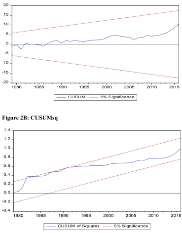
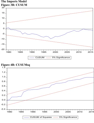
The test will favor the presence of cointegration between the variables if the computed ARDL-F statistic is more than the upper critical bound. However, the decision would be no cointegration between the variables if the lower critical bound is greater than the calculated ARDL-F statistic and would be inconclusive if the computed ARDL-F statistic is between the lower and upper critical bounds. We use the critical bounds generated by Narayan (2005) because the data sample is small (i.e. 54 observations) and in this case the critical bounds tabulated by Pesaran et al. (2001) are not suitable. The stability of the bounds testing approach estimated is tested by applying CUSUM and CUSUMsq suggested by Brown et al. (1975).

We apply the ARDL bounds testing approach in order to examine the presence of cointegration between the variables. If the existence of cointegration between the variables is confirmed, we then estimate the long-run impact of economic growth (Yt), biomass energy consumption (Et), oil prices (Ot) and trade openness (TRt) on carbon emissions (Ct) by following Equation (5):

i t t

t t

t t t

t Y Y Y E O TR TR

C    _ _     2

6 5

4 3

3 1 2

1 2 1

0 ln ln [ ] ln ln ln ln

ln (5)

where

1 6

1 5

1 4

1 3

1 ] [ 2

1 1

1

0  / ,  / ,  2 3 / ,  / ,  / ,  / ,  2/

  _C  _Y  _Y _Y  _E  _O  _TR  _TR

and_t_{is the error term assumed of having normal distribution. We apply a similar approach}

with various proxies of trade openness (exports, imports, trade) to examine the association between CO2 emissions, economic growth, biomass energy consumption, oil prices and trade

openness for the U.S. economy.

4.2 The VECM Granger causality approach

(20)

19                                                                                                                                      



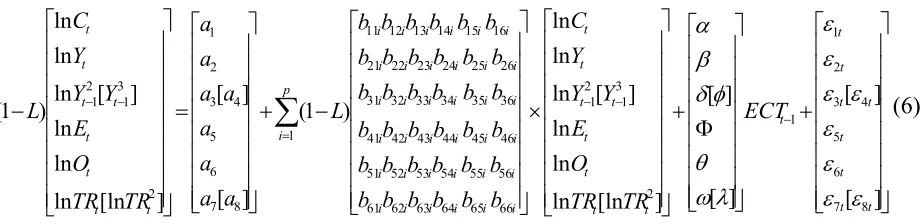
] [ ] [ ] [ ] [ ] [ln ln ln ln ] [ ln ln ln ) 1 ( ] [ ] [ ] [ln ln ln ln ] [ ln ln ln ) 1 ( 8 7 6 5 4 3 2 1 1 2 3 1 2 1 66 65 64 63 62 61 56 55 54 53 52 51 46 45 44 43 42 41 36 35 34 33 32 31 26 25 24 23 22 21 16 15 14 13 12 11 1 8 7 6 5 4 3 2 1 2 3 1 2 1 t t t t t t t t t t t t t t t t t i i i i i i i i i i i i i i i i i i i i i i i i i i i i i i i i i i i i p i t t t t t t t t ECT TR TR O E Y Y Y C b b b b b b b b b b b b b b b b b b b b b b b b b b b b b b b b b b b b L a a a a a a a a TR TR O E Y Y Y C L                (6)

where (1L)_{is the difference operator. The lagged residual term i.e.}ECTt-1 is derived from the

long-run relationship. The error terms are shown by 1t,2t,3t,4t,5t,6t,7t and8t. The long-run causality is derived from the significance value of the coefficient forECMt1 through using

the t-test statistic. The direction of the short-run causality between the variables is judged through using the F-statistic for the first differenced lagged independent variables.

[image:20.612.76.536.91.203.2]

6. Empirical results

Table 2 presents the descriptive statistics and the historical correlation analysis. We note that all the variables have normal distributions as confirmed by the Jaque-Bera test. In the correlation analysis, the presence of negative correlation is noted between biomass energy consumption and CO2 emissions, indicating that this renewable energy consumption lowers

carbon missions due to the absorption of CO2 emissions by new tree growth. On the other hand,

a positive correlation exists between economic growth and CO2 emissions. Further, oil prices and

CO2 emissions are positively correlated. The correlations of exports, imports and trade with CO2

(21)

20

Table-2: Descriptive statistics and correlation analysis

Variables ln Ct ln Et ln Yt ln Ot lnTRt lnEXt lnIMt Mean 2.9543 16.1201 10.3118 3.6190 8.0047 7.2466 7.3632 Median 2.9626 16.2037 10.3688 3.5973 8.3148 7.5057 7.7257 Maximum 3.1139 16.5582 10.7802 4.7468 9.9645 9.1528 9.3773 Minimum 2.7042 15.7242 9.6252 2.3786 4.6319 4.2223 3.5415 Std. Dev. 0.0821 0.2602 0.3392 0.7523 1.3873 1.3028 1.4726 Skewness -0.7035 -0.2402 -0.3305 -0.1123 -0.5188 -0.4736 -0.5786 Kurtosis 3.9470 1.7445 1.9400 1.7531 2.1741 2.0998 2.3177 Jarque-Bera 4.0322 4.2916 3.7063 3.8122 4.1776 4.0558 4.2865 Probability 0.1328 0.1169 0.1567 0.1486 0.1238 0.1316 0.1172

t C

ln _1.0000

t E

ln _{-0.0298 1.0000}

t Y

ln _{0.1881 0.4272} _1.0000

t O

ln 0.1318 0.3560 -0.3575 1.0000 t

TR

ln _{-0.1918 0.5728} _{0.4586 -0.5290 1.0000}

t EX

ln _{-0.1804 0.6762} _{0.5465 -0.4300 0.9991 1.0000}

t IM

ln _{-0.2067 0.4682} _{0.4980 -0.3266 0.9992 0.9968 1.0000} Note: Ct is CO2 emissions per capita, Et is biomass energy consumption per capita,

Yt is real GDP per capita, Ot is real oil prices, EXt is exports, IMt is imports and TRt

is trade.

In order to examine the unit root properties of the variables, we have applied the Ng-Perron unit root test (2001) which provides efficient empirical results for small samples such as in our case7. The empirical results indicate that all the series are non-stationary in the level by using the intercept and time trend but are stationary in the first difference of the variables8_{. The}

Ng-Perron unit root test provides ambiguous empirical results due to their low explanatory power since this unit root test does not accommodate information about unknown structural break dates stemming from the series, which further weakens the stationarity hypothesis.

To resolve this issue, we employ the Clemente-Montanes-Reyes (1998) unit root test which contains information about single and double unknown structural breaks occurring in the

7_{Testing the unit root properties of a variable is necessary to apply any standard cointegration methods such as the}

bounds testing or the Johansen methods to cointegration.

8_{We have not provided the results of the Ng-Perron (2001) unit root test to conserve space but they are available}

(22)

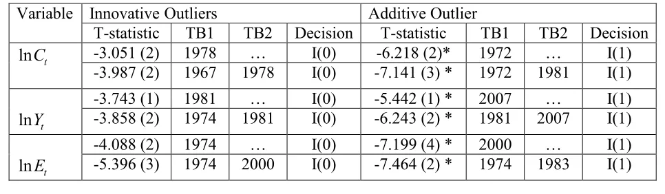
21 series during the sample period. Table 3 details the results of the CMR (Clemente-Montanes-Reyes) unit root test. We note that the variables are non-stationary in the level in the presence of structural breaks. The structural breaks are found in CO2 emissions, economic growth, biomass

energy consumption, oil prices, trade openness, exports and imports for the years of 1978, 1981, 1974, 1971 and 1970, respectively. These years are associated with major events in the economy and the oil market. For example, 1973-1974 are the years of OPEC oil embargo, 1980 is a year of a major economic recession in the United States. The break point in 1978 for carbon emissions signifies the implementation of Water Pollution Control Act Amendments (WPCAA, 1977) which is also commonly known as Superfund Act in 1980 (SA, 1980). This act helped in regulating public drinking water systems, toxic substances, pesticides, and ocean dumping; and protected wildlife, wilderness, and wild and scenic rivers. This series of new laws provided for conducting pollution research, improve standard setting, contaminated site cleanup, monitoring, and enforcement. We may conclude that the implementation of WPCAA not only affected energy but also environmental quality in 1978.

[image:22.612.70.553.532.673.2]

We note that all the variables are stationary in their first difference form. This indicates that all the series are integrated of I(1). The robustness of stationarity properties of the variables is checked by applying the CMR (1998) test that accounts for information for double unknown structural breaks in the series. The results display in Table 3 unveil that all the series have a unit root problem in the level but show stationary in the first difference. It is noted that all the variables have unique order of integration9_.

Table 3: Unit root analysis with structural breaks

Variable Innovative Outliers Additive Outlier

T-statistic TB1 TB2 Decision T-statistic TB1 TB2 Decision t

C

ln -3.051 (2) 1978 … I(0) -6.218 (2)* 1972 … I(1)

-3.987 (2) 1967 1978 I(0) -7.141 (3) * 1972 1981 I(1)

t Y

ln -3.743 (1) 1981 -3.858 (2) 1974 1981 … I(0) I(0) -5.442 (1) * -6.243 (2) * 2007 1981 2007 … I(1) I(1)

t E

ln -4.088 (2) 1974 -5.396 (3) 1974 2000 … I(0) I(0) -7.199 (4) * -7.464 (2) * 2000 1974 1983 … I(1) I(1)

9_{The graphical presentation of CMR unit root test with indication of structural break is given in Appendix-A for all}

(23)

22 t

O

ln -2.710 (2) 1971 -3.470 (3) 1977 2009 … I(0) I(0) -7.247 (3) * 6.609 (2) * 1977 1977 1996 … I(1) I(1)

t TR

ln -2.920 (1) 1971 _{-4.162 (2) 1971 1992}… I(0) _I(0) -14.496 (1) * 1979 _{-17.236 (2) * 1979 2008}… I(1) _I(1)

t EX

ln _{-3.959 (2) 1971 1985}2.122 (3) 1971 … I(0) _I(0) -11.343 (2) * 1979 _{-11.728 (1) * 1970 1979}… I(1) _I(1)

t IM

ln -3.029 (2) 1970 _{-4.616 (2) 1971 1992}… I(0) _I(0) -16.579 (2) * 1979 _{-9.703 (3) *} _{1979 2008}… I(1) _I(1) Note: * and** represent significance at the 1% and 5% levels, respectively. () shows the lag length of the variables. TB1 and TB2 refer to structural break dates.

(24)

[image:24.792.89.706.100.517.2]

23

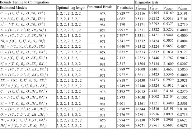
Table 4: The results of the ARDL cointegration test

Bounds Testing to Cointegration Diagnostic tests

Estimated Models Optimal lag length Structural Break F-statistics 2

NORMAL  2 ARCH  2 RESET  2 SERIAL  ) , , , , ,

( 2 2

t t t t t t

t f Y Y E O TR TR

C  _{2, 2, 1, 2, 2, 2, 2} ₁₉₇₈ _{6.829 ** 0.3116 1.9105 1.8169 2.5191}

) , , , , ,

( 2 2

t t t t t t

t f C Y E O TR TR

Y  _{2, 2, 2, 1, 2, 2, 1} ₁₉₈₁ _4.062 _{0.5111 0.2212 0.5518 4.7101}

) , , , , , ( 2 2 t t t t t t

t f Y C E O TR TR

Y  _{2, 2, 2, 1, 2, 2, 2} ₁₉₈₁ _4.170 _{0.1171 0.3292 0.5373 1.2710}

) , , , , ,

( 2 2

t t t t t t

t f C Y Y O TR TR

E  _{2, 2, 2, 2, 2, 1, 2} ₁₉₇₄ _{6.997 *} _{1.2311 2.1322 2.5252 0.4000}

) , , , , ,

( 2 2

t t t t t t

t f C Y Y E TR TR

O  _{2, 2, 2, 1, 1, 2, 2} ₁₉₇₁ _{7.797 *} _{1.3311 2.1421 1.5441 0.4000}

) , , , , ,

( 2 2

t t t t t t

t f C Y Y E O TR

TR  _{2, 2, 2, 2, 2, 2, 2} ₁₉₇₁ _{6.341 ** 0.1332 0.3424 0.5055 0.4004}

) , , , , , ( 2 2 t t t t t t

t f C Y Y E O TR

TR  _{2, 2, 2, 2, 2, 2, 2} ₁₉₇₁ _{6.640 ** 0.1312 0.3224 0.5657 0.4074}

) , , , , ,

( 2 2

t t t t t t

t f Y Y E O EX EX

C  _{2, 2, 1, 2, 2, 2, 2} ₁₉₇₈ _{8.837 *} _{0.6313 2.6332 0.1831 1.9127}

) , , , , ,

( 2 2

t t t t t t

t f C Y E O EX EX

Y  _{2, 2, 2, 1, 2, 2, 1} ₁₉₈₁ _2.112 _{1.2323 1.3446 2.1762 0.9012}

) , , , , , ( 2 2 t t t t t t

t f Y C E O EX EX

Y  _{2, 2, 2, 1, 2, 2, 2} ₁₉₈₁ _2.317 _{1.1304 0.3134 2.1609 0.8207}

) , , , , ,

( 2 2

t t t t t t

t f C Y Y O EX EX

E  _{2, 2, 2, 2, 2, 1, 2} ₁₉₇₄ _{7.789 ** 0.1608 0.3401 1.4653 1.5850}

) , , , , ,

( 2 2

t t t t t t

t f C Y Y E EX EX

O  _{2, 2, 2, 1, 1, 2, 2} ₁₉₇₁ _{7.927 *} _{1.3611 2.3423 1.5346 0.4000}

) , , , , ,

( 2 2

t t t t t t

t f C Y Y E O EX

EX  _{2, 2, 2, 2, 2, 2 , 2} ₁₉₇₁ _{9.818 *} _{0.2430 0.4423 0.2929 2.3021}

) , , , , , ( 2 2 t t t t t t

t f C Y Y E O EX

EX  _{2, 2, 2, 2, 2, 2 , 2} ₁₉₇₁ _{6.749 ** 0.2140 0.3324 0.1912 2.3021}

) , , , , ,

( 2 2

t t t t t t

t f Y Y E O IM IM

C  _{2, 2, 1, 2, 2, 2, 2} ₁₉₇₈ _{6.395 ** 0.2015 2.4181 2.4161 0.2370}

) , , , , ,

( 2 2

t t t t t t

t f C Y E O IM IM

Y  _{2, 2, 2, 1, 2, 2, 1} ₁₉₈₁ _2.873 _{0.3050 1.2002 2.2104 0.1502}

) , , , , , ( 2 2 t t t t t t

t f Y C E O IM IM

Y  _{2, 2, 2, 1, 2, 2, 2} ₁₉₈₁ _3.901 _{1.1561 0.1221 0.3480 2.5501}

) , , , , ,

( 2 2

t t t t t t

t f C Y Y O IM IM

E  _{2, 2, 2, 2, 2, 1, 2} ₁₉₇₄ _{7.670 ** 0.6344 0.4316 1.5191 2.8101}

) , , , , ,

( 2 2

t t t t t t

t f C Y Y E IM IM

O  _{2, 2, 2, 1, 1, 2, 2} ₁₉₇₁ _{7.476 ** 0.7891 0.8976 1.8971 0.8716}

) , , , , ,

( 2 2

t t t t t t

t f C Y Y E O IM

IM  _{2, 2, 2, 2, 2, 2 , 2} ₁₉₇₀ _{7.974 ** 0.9130 0.2949 1.2901 2.6627}

) , , , , , ( 2 2 t t t t t t

t f C Y Y E O IM

(25)

24 ) , , , , , ,

( 2 3 2

t t t t t t t

t f Y Y Y E O TR TR

C  _{2, 2, 1, 2, 2, 2, 2} ₁₉₇₈ _{9.151 *} _{1.6564 0.1613 2.4080 0.2502}

) , , , , , ,

( 2 3 2

t t t t t t t

t f C Y Y E O TR TR

Y  2, 2, 2, 1, 2, 2, 1 ₁₉₈₁ _3.701 _{1.8464 0.1313 2.4811 0.2501}

) , , , , , ,

( 3 2

2 t t t t t t t

t f C Y Y E O TR TR

Y  _{2, 2, 2, 1, 2, 2, 2} ₁₉₈₁ _2.105 _{1.6040 0.1260 2.3801 0.0221}

) , , , , , ,

( 2 2

3 t t t t t t t

t f C Y Y E O TR TR

Y  _{2, 2, 2, 1, 2, 2, 2} ₁₉₈₁ _3.272 _{1.4049 0.1409 2.3038 0.1245}

) , , , , , ,

( 2 3 2

t t t t t t t

t f C Y Y Y O TR TR

E  _{2, 2, 2, 1, 1, 2, 2} ₁₉₇₄ _{6.538 ** 1.4044 0.4609 2.3679 0.1450}

) , , , , , ,

( 2 3 2

t t t t t t t

t f C Y Y Y O TR TR

P  _{2, 2, 2, 2, 2, 2, 2} ₁₉₇₁ _{8.901 *} _{0.8976 0.8765 0.5436 0.3456}

) , , , , , ,

( 2 3 2

t t t t t t t

t f C Y Y Y E O TR

TR  _{2, 2, 2, 2, 2, 2, 2} ₁₉₇₁ _9.231* _{2.1421 1.0309 2.4260 1.1550}

) , , , , , ,

( 2 3

2 t t t t t t t

t f C Y Y Y E O TR

TR  _{2, 2, 2, 2, 2, 2, 2} ₁₉₇₁ _{9.018 *} _{1.0989 0.8971 1.0879 0.8956}

) , , , , , ,

( 2 3 2

t t t t t t t

t f Y Y Y E O EX EX

C  2, 2, 1, 2, 2, 2, 2 ₁₉₇₈ _{9.135 *} _{2.3431 2.0204 2.6525 2.3635}

) , , , , , ,

( 2 3 2

t t t t t t t

t f C Y Y E O EX EX

Y  2, 2, 2, 1, 2, 2, 1 ₁₉₈₁ _3.751 _{1.2810 0.4202 2.1432 0.3501}

) , , , , , ,

( 3 2

2 t t t t t t t

t f C Y Y E O EX EX

Y  _{2, 2, 2, 1, 2, 2, 2} ₁₉₈₁ _2.112 _{1.3212 0.3202 2.4142 0.5303}

) , , , , , ,

( 2 2

3 t t t t t t t

t f C Y Y E O EX EX

Y  _{2, 2, 2, 1, 2, 2, 2} ₁₉₈₁ _3.070 _{1.1209 0.3602 2.3434 0.2124}

) , , , , , ,

( 2 3 2

t t t t t t t

t f C Y Y Y O EX EX

E  _{2, 2, 2, 1, 1, 2, 2} ₁₉₇₄ _{6.598 ** 2.0409 1.3209 1.4060 1.0313}

) , , , , , ,

( 2 3 2

t t t t t t t

t f C Y Y Y O EX EX

P  _{2, 2, 2, 2, 2, 2, 2} ₁₉₇₁ _{8.808 *} _{1.1010 2.1021 2.4302 2.2130}

) , , , , , ,

( 2 3 2

t t t t t t t

t f C Y Y Y E O EX

EX  2, 2, 2, 2, 2, 2, 2 ₁₉₇₁ _9.131* _{1.2102 2.2003 1.4021 2.0312}

) , , , , , ,

( 2 3

2 t t t t t t t

t f C Y Y Y E O EX

EX  _{2, 2, 2, 2, 2, 2, 2} ₁₉₇₁ 9.218 * 1.0261 1.0203 2.1011 0.1021

) , , , , , ,

( 2 3 2

t t t t t t t

t f Y Y Y E O IM IM

C  2, 2, 1, 2, 2, 2, 2 ₁₉₇₈ _{9.445 *} _{0.6302 0.1032 2.2035 0.5032}

) , , , , , ,

( 2 3 2

t t t t t t t

t f C Y Y E O IM IM

Y  _{2, 2, 2, 1, 2, 2, 1} ₁₉₈₁ _2.075 _{1.2040 0.2023 2.3031 0.2030}

) , , , , , ,

( 3 2

2 t t t t t t t

t f C Y Y E O IM IM

Y  2, 2, 2, 1, 2, 2, 2 ₁₉₈₁ _3.132 _{2.2101 1.1301 0.6515 0.0552}

) , , , , , ,

( 2 2

3 t t t t t t t

t f C Y Y E O IM IM

Y  _{2, 2, 2, 1, 2, 2, 2} ₁₉₈₁ _3.175 _{1.2152 1.0050 0.2519 0.5305}

) , , , , , ,

( 2 3 2

t t t t t t t

t f C Y Y Y O IM IM

E  _{2, 2, 2, 1, 1, 2, 2} ₁₉₇₄ _{7.190 ** 0.8970 0.9817 0.1234 0.9801}

) , , , , , ,

( 2 3 2

t t t t t t t

t f C Y Y Y O IM IM

P  _{2, 2, 2, 2, 2, 2, 2} ₁₉₇₁ _{8.868 *} _{0.7654 0.2389 0.8712 0.2348}

) , , , , , ,

( 2 3 2

t t t t t t t

t f C Y Y Y E O IM

IM  _{2, 2, 2, 2, 2, 2, 2} ₁₉₇₀ _{9.535 *} _{0.1978 0.4567 0.0980 0.1350}

) , , , , , ,

( 2 3

2 t t t t t t t

t f C Y Y Y E O IM

IM  _{2, 2, 2, 2, 2, 2, 2} ₁₉₇₀ _{9.458 *} _{0.3457 0.8912 0.6780 0.8017}

(26)

25 Lower bounds I(0) Upper bounds I(1)

7.227 8.340

5.190 6.223

4.370 5.303

(27)

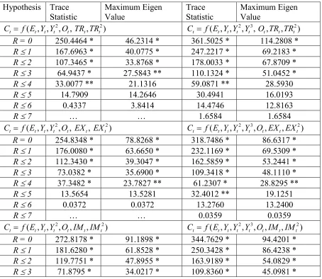
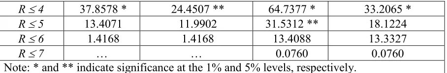
26 We find a unique level of integration for all variables, so we can move to apply the Johansen and Juselius, (1990) maximum likelihood cointegration test in order to test the robustness of cointegration results. The results of Johansen cointegration test reported in Table 4 reveal that the null hypothesis of no cointegration is rejected because the trace statistic and maximum Eigen value show the presence of one cointegrating vector between the variables as we measure trade openness by exports, imports and trade using squared and cubic functions of carbon emissions. The presence of a cointegrating vector confirms the existence of a long-run cointegration between the variables. This finding underscores the robustness of the empirical results of a long-run cointegration association between the variables.

[image:27.612.81.535.304.698.2]

Table 5: Results of the Johansen cointegration tests with squared and cubic specifications

Hypothesis Trace

Statistic Maximum Eigen Value Trace Statistic Maximum Eigen Value ) , , , , ,

( 2 2

t t t t t t

t f E Y Y O TR TR

C  ( , , 2, 3, , , 2)

t t t t t t t

t f E Y Y Y O TR TR C 

R = 0 250.4464 * 46.2314 * 361.5025 * 114.2808 * R  1 167.6963 * 40.0775 * 247.2217 * 69.2183 * R  2 107.3465 * 33.8768 * 178.0033 * 67.8709 * R  3 64.9437 * 27.5843 ** 110.1324 * 51.0452 *

R  4 33.0077 ** 21.1316 59.0871 ** 28.5930

R  5 14.7909 14.2646 30.4941 16.0193

R  6 0.4337 3.8414 14.4746 12.8163

R  7 … … 1.6584 1.6584

) , , , , ,

( 2 2

t t t t t t

t f E Y Y O EX EX

C  ( , , 2, 3, , , 2)

t t t t t t t

t f E Y Y Y O EX EX C 

R = 0 254.8348 * 78.8268 * 318.7486 * 86.6317 * R  1 176.0080 * 63.6650 * 232.1169 * 69.5309 * R  2 112.3430 * 39.3047 * 162.5859 * 53.2441 *

R  3 73.0382 * 35.6900 * 109.3418 * 48.1110 *

R  4 37.3482 * 23.7827 ** 61.2307 * 28.8295 **

R  5 13.5654 13.5281 32.4012 ** 19.1251

R  6 0.0372 0.0372 13.2760 13.2400

R  7 … … 0.0359 0.0359

) , , , , ,

( 2 2

t t t t t t

t f E Y Y O IM IM

C  ( , , 2, 3, , , 2)

t t t t t t t

t f E Y Y Y O IM IM C 

R = 0 272.8178 * 91.1898 * 344.7629 * 94.4201 * R  1 181.6280 * 61.8528 * 250.3428 * 86.4238 * R  2 119.7751 * 47.8955 * 163.9189 * 54.0829 *

(28)

27

R  4 37.8578 * 24.4507 ** 64.7377 * 33.2065 *

R  5 13.4071 11.9902 31.5312 ** 18.1224

R  6 1.4168 1.4168 13.4088 13.3327

R  7 … … 0.0760 0.0760

Note: * and ** indicate significance at the 1% and 5% levels, respectively.

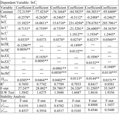
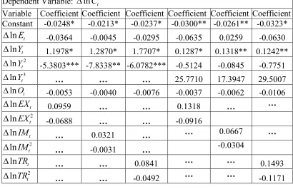
The presence of cointegration between the variables paves the way to examine the long-run and short-long-run dynamic relationships between the variables. The long-long-run results reported in Table 6 show that biomass energy consumption has a negative impact on carbon emissions, which highlights that biomass energy is good for the environment. For instance, we observe that a 1% increase in biomass energy consumption will decrease emissions by 0.25-0.31%. This evidence is similar to that found by Bilgili et al. (2016) and Bilgili (2016) for the US economy.

Oil prices are positively and significantly linked with carbon emissions. This finding implies that oil prices increase CO2 emissions. A 1% rise in those prices leads carbon emissions

to increase by 0.03-0.04%. This empirical evidence is consistent with the results of Chai et al. (2016), which indicate that higher oil prices make firms use other fossil fuel substitutes such as dirty coal that increase carbon emissions.

The association between economic growth and carbon emissions has an inverted U-shaped when exports, imports and trade are used as measures of trade openness. We find that a 1% increase in real GDP would increase carbon emissions by 15.10%-16.06%, using the three different measures of trade openness. The negative sign of the squared term of real GDP in the carbon emissions function corroborates the delinking of carbonemissions at a higher level of real GDP, while again controlling for exports, imports and trade as measures of trade openness. This is evidence for the existence of EKC in the United States. This empirical evidence is similar to that of Unruh and Moomaw (1998) and Roach (2013) which underscores the presence of the EKC hypothesis for the US economy.

The relationship between trade openness (as measured by exports, imports and trade) and carbon emissions has a U-shaped. We note that exports (imports) have a negative and significant impact on CO2 emissions, suggesting that international trade is good for the environment. A 1%

[image:28.612.81.535.71.146.2]

(29)

28 (exports, imports and trade) also corroborates the positive linking of carbon emissions with trade openness at a higher level of real trade, while controlling biomass energy consumption, oil prices and economic growth. This finding is evidence of the existence of a U-shaped association between trade openness and carbon emission in the United States10_{. The dummy variable has a}

[image:29.612.101.512.266.674.2]

positive and significant effect on carbon emissions. This shows that the implementation of Water Pollution Control Act Amendments (WPCAA) could not improve the environmental quality by lowering CO2 emissions in the US economy.