Index Terms Human face authentication; Gabor wavelets;



Abstract—Two facial authentication methods based on two different Gabor phase feature representations are proposed in this paper. In the first proposed scheme, similarity score having the highest classification accuracy is used as threshold of the Gabor filter. In the second method, minimum intra-personal similarity score is used as individual subject’s threshold for authentication. Both of these methods have shown high classification capability for our dataset.

Index Terms--Human face authentication; Gabor wavelets; Gabor magnitude features; Local Gabor binary pattern.

I. INTRODUCTION

Due to unconstrained variations of pose, illumination, key frame selection and region of interest, automated real time face authentication is a challenging objective. The fast and automatic method of face authentication is to use a class specific threshold on the similarity measure when verifying the face image. On the basis of the threshold, the authentication system should accept the query image as a positive sample or reject it. Due to the difficulty level in face authentication problems, the selection of proper threshold of a given class in a dataset is an open problem because this difficulty level can change in different situations e.g. in video surveillance issues. The determination of the threshold is usually done by using receiver operating characteristic (ROC) curve which is based on the different values of false positive rate (FPR) and true positive rate (TPR) [1] as mentioned by Mansfield et al. [2]. Generally, the point on the ROC curve that has the maximum accuracy, i.e. TPR-FPR value, is selected as the operating threshold. We call this method the global threshold which provides a binary classification threshold between negative and positive set. However, for multiclass classification problem, individual threshold of each class can be used. We call this the local threshold approach.

Manuscript received December 27, 2012; revised January 22, 2013. This work is supported by G4S Security Services Bangladesh (P) Ltd (http://www.g4s.com.bd/).

Iqbal Nouyed is with the Computer Vision & Cybernetics Research, SECS, Independent University, Bashundhara, Dhaka 1229, Bangladesh (e-mail: [email protected]).

Bruce Poon is with the School of Electrical & Information Engineering, University of Sydney, NSW 2006, Australia (e-mail: [email protected]).

Ashraful Amin is with the Computer Vision & Cybernetics Research, SECS, Independent University, Bashundhara, Dhaka 1229, Bangladesh. (e-mail: [email protected]).

Hong Yan is with the Department of Electronic Engineering, City University of Hong Kong, Hong Kong, China (e-mail:[email protected])

In this paper, we evaluate the performance of these two face authentication methods for two different Gabor phase based feature representations. The proposed threshold based face verification methods and the experimental results are described in subsequent sections.

II. THEFACEAUTHENTICATIONSYSTEM In face verification systems, the user makes a “positive” claim to an identity, requiring a “one-to-one” comparison of the submitted face sample to the enrolled face template of the claimed identity. The procedure is shown in Figure 1.

Figure 1. A typical face authentication system These components are discussed in following sections .

A. Face data acquisition

To evaluate the performance of the proposed system, images from our in-house database are being used. The in-house database contains images which were collected using a generic webcam. Most of the images were taken from a 100 frame video sequence recorded in unconstrained environment where illumination, background and facial expression were not restricted. However, the distance from camera and face orientation was kept consistent in all recordings. Video sequences of a total of 60 subjects were collected. The images taken were of size 352×440.

In Figure 2, sample images from the database are shown for reference.

Figure 2. Sample images from the in-house database

Facial Authentication using Gabor Phase Feature

Representations

B. Face data preprocessing

We use Viola-Jones Ada Boosted algorithm [3] to extract the face region from the image. This algorithm has become almost a de facto standard for face detection from images taken in unconstrained environment. As per requirement of the algorithm, all the images we have used contain full frontal upright faces. The basic principle of the Viola-Jones algorithm is to scan a sub-window capable of detecting faces across a given input image. It rescales the detector and runs it many times through the image at different sizes each time. This scale invariant detector is constructed using an integral image and simple rectangular features of Haar wavelets. In Figure 3, a gray level raw image of size 256×354 is cropped and resized into a 128×128 facial region image after face detection. After that, the intensity of the image is normalized.

Figure 3. Extraction of face region from a video frame and preprocessing

C. Facial feature extraction

Facial features are acquired in a few steps. Firstly, Gabor wavelet is applied on the cropped facial region image and phase of each of the filter responses is calculated. For each of the Gabor phase face, local Gabor binary pattern (LGBP) [4] is calculated. After that, each of the LGBP image is divided into smaller non overlapping regions and histograms are calculated for each of the regions [5]. Finally, these local histograms are concatenated one after another to construct the final feature vector.

1) The Gabor wavelet

Due to their biological relevance and computational properties, Gabor wavelets are introduced to image analysis. As a feature generator, Gabor filters are widely used in face recognition. Since the kernels of Gabor wavelets are similar to the 2D receptive field profiles of the mammalian cortical simple cells, they exhibit desirable characteristics of spatial locality and orientation selectivity. They are also optimally localized in the space and frequency domains. The Gabor wavelets (kernels, filters) can be defined as follow [5]:

, , ,

‖ ‖

, (1)

where v and μ define the scale and orientation of the Gabor kernel, z denotes the pixel, i.e., z=(x,y); ‖∙‖ denotes the Euclidean norm operator, and the wave vector , is defined as:

, (2)

where /8 is the orientation parameter and k k /f , where f is the spacing factor between filters in the

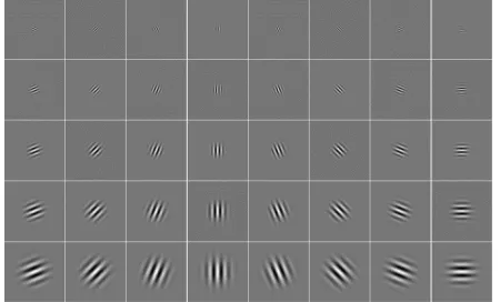
frequency domain. In Figure 4, Gabor kernels at five different scales and eight different orientations are depicted.

Given an input face image I, its convolution with Gabor wavelet ψ , can be defined as:

, ∗ , (3)

where * denotes the convolution operator. For each Gabor kernel, at every image pixel z, a complex number containing a real part and an imaginary part is generated. Based on these two parts phase Φ , z can be computed as follow:

Φ , ,

, (4)

In our work, Gabor filters at five scales (v={0,1,…,4} in Equation (1)), and eight orientations (μ={0,1,2,…,7} ranging between 0° _{to 7π/8}° _{in Equation (1)) are applied on each} preprocessed facial image.

Figure 4. Real part of Gabor kernels at 5 scales (v={0,1,…,4}) and 8 orientations (μ={0,1,2,…,7})

Here note that the preprocessed image is 128×128 and the scale size is relative to this image size. The Gabor filters exhibit some invariance to background, translation, distortion and size. However, this invariance property of the Gabor wavelet may not hold if the change in background, translation, distortion or size is too large. In this sense the filter scale and image size is related. By convolving the Gabor filters/kernels with the facial image, the Gabor filter/kernel representation of a facial image is obtained. Therefore, 40 Gabor responses are recorded from a single facial image. Figure 5 presents 40 Gabor phase representation of the normalized facial image of Figure 3 for the values σ=2π, =π/2, and f=√2 in Equation (1).

2) Local Gabor Binary Pattern Histogram Sequence (LGBPHS)

discriminating power. It is based on multi-resolution spatial histogram combining local intensity distribution with the spatial information. Therefore, it is robust to noise and local image transformations due to variations of lighting, occlusion and pose. In LGBPHS, a face image is modeled as a “histogram sequence” by dividing each local Gabor binary pattern (LGBP) [4] map into non-overlapping rectangle regions with specific size, and histogram is computed for each region. The LGBP histograms of all the LGBP maps are then concatenated to form the final histogram sequence as the model of the face.

Figure 5. Gabor phase representation of the face of Figure 3 (shown as a fourth order tensor)

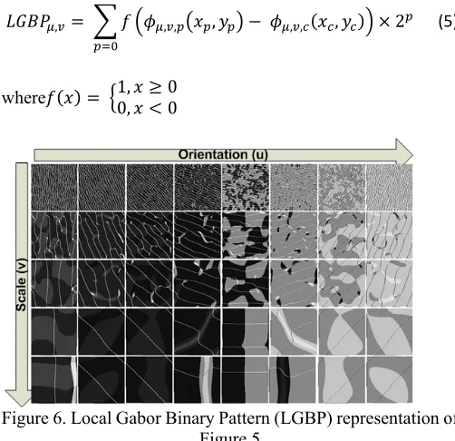
Local Gabor binary pattern (LGBP) operator based on Gabor phase labels the pixels of Gabor phase image by calculating neighborhood of each pixel with center value through Equation (5). After LGBP calculation, the Gabor phase images of Figure 5 looks like one presented in Figure 6. If eight neighborhoods of the center pixel, located at x , y , are x , y , where p=0,1,…,7, then LGBP based on Gabor phase at x , y is defined as follows [4]:

, , , , , , , 2 (5)

where 1,_0, 0₀

Figure 6. Local Gabor Binary Pattern (LGBP) representation of Figure 5

These LGBP labels are then encoded further to local histograms, which are used as face representation for classification. If each LGBP map is divided into R

non-overlapping regions, then histogram of rth region of specific LGBP map (from (v,μ)th Gabor phase picture) is computed by:

, , , , 0 , , , 1 , … , , , 1 (6)

where T is the bin size. Then all the histogram pieces computed from the R regions of a LGBP map are concatenated to a histogram sequence of LGBP image as follows:

, , , , , , , … , , , (7)

3) The Gabor feature representation

The result of a Gabor transformation can be seen as a fourth order tensor TG(u,v,l,m) (Figure 5) which is a 8×5×128×128 tensor in this example, where u={1,2,…,8},v={1,2,…,5} are indexes along orientation and scale of Gabor filter response and l={1,2,…,128) and m={1,2,…,128} are width and height of the image respectively. It can be noticed that entries of the fourth order tensor are complex numbers and the phase part of this fourth order tensor is defined here as the Gabor phase-face which we can acquire using Equation (4). There are 40 components (Gabor phase-face) for a single facial image in Gabor facial representation, and each one is the phase part of the output which is obtained by convolving a facial image with 40 Gabor filters/kernels.

In the conventional representation, the output of a Gabor function using the convolution I x, y ∗ ψ , x, y (Equation (3)) followed by application of LGBPHS will return a histogram based basic Gabor-phase feature vector for the μth orientation at vth scale, and dimension of this vector is n=256×l/16×m/16=256×8×8=16384. It is because during LGBPHS (Equation (7)) calculation, 64 non overlapping regions are considered. It means that in Equation (7), value for R=8×8=64 is chosen. LGBP contains values ranging between [0, 255] since the bin size of T=256 is chosen in Equation (5).

4) 40 basic Gabor filter and summed Gabor filter of all scale and orientations

We used each of the 40 different Gabor face as 40 different representation of a single face image. Instead of using Equation (8), we use the following formula:

, , 8

where , is the Gabor feature vector for filter response of Gabor filter/kernel at μ orientation and v scale. From this, it can be seen that 40 different representations are possible for a single facial image.

The sum of Gabor representations in all scales and all orientations is:

∑,∑ ∗ , ∗ ,

∑,∑ arctan ∑,∑

∑,∑

∑,∑, ∑,∑, 0 , ∑,∑, 1 , … , ∑,∑, 1

∑,∑ ∑,∑, , ∑,∑, , … , ∑,∑, 9 where, ∑,∑ is the Gabor feature vector. In this representation filter responses for all orientations for a scale is summed and then each such representation of scale is summed.

5) Similarity measure

As the number of samples per subject is only a few for the databases, distance based similarity measures are employed to identify persons in the gallery database. Here notice that using LGBPHS, facial images are represented as histogram sequences. Similarity of two faces represented can be calculated as:

, ,, , ,, … , , , , , , , … , , , , , ,, … , , ,

and , ,, , , , … , , , , , ,, … , , , , , ,, … , , , ).To calculate their matching score, histogram intersection is applied. Histogram intersection of two histograms, denoted as

∩ h , h , is used as a similarity measurement of two

histograms can be defined as follows [6]:

∩ , min , (10)

where h and h are two histograms, and T is the number of bins in the histogram. The intuitive motivation for this measurement is calculation of the common part of two histograms. Using histogram intersection the similarity of two face images based on the LGBPHS face representation is computed by:

∩ , ∩ , , , , , (11)

D. Face Authentication

For our face authentication system we applied two types of thresholds, 1) Global threshold, and 2) Local threshold.

1) Global Threshold

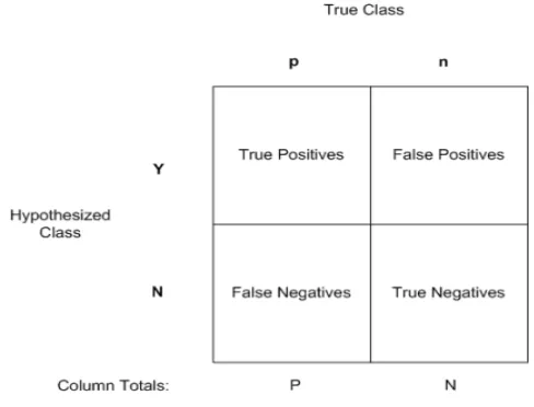
When considering a global threshold, we are solving a classification problem between two classes. In such case, each instance is mapped to one element of the set , of positive and negative class labels. The classification model maps from instance to predicted classes. Given a classifier and an instance, there are four possible outcomes. If the instance is positive and it is classified as positive, it is counted as a true positive (TP).If it is classified as negative, it is counted as false negative (FP). If the instance is negative and it is classified as negative, it is counted as true negative (TN); if it is classified as positive, it is counted as a false positive (FN). Given a classifier and a set of instances (the test set), a two-by-two confusion matrix (also called a contingency table) can be constructed representing the dispositions of the set of instances. Given a classifier and a set of instances (the test set), a two-by-two confusion matrix (also called a contingency table) can be constructed representing the dispositions of the set of instances.

The numbers along the major diagonal represent the correct decision made, and the numbers off the diagonal represent the errors (confusion) between the various classes.

Figure 7 shows a confusion matrix. We picked the similarity

measure that provides the highest accuracy for both , and ∑,∑ based feature representations as the global threshold, where accuracy is calculated as [1]:

12

where, TP = true positive, TN = true negative, P = number of positive samples, and N = number of negative samples.

Figure 7.The confusion matrix.

Moreover, equations of several common metrics that we calculated from the confusion matrix are the true positive rate:

tp rate ≈Positives correctly classified / Total positives and the false positive rate :

fp rate ≈Negatives incorrectly classified / Total negatives By using these two equations, we can construct the ROC curve that can help us to find the optimal threshold for the training set. It is a two-dimensional graph of which TP rate is plotted on the Y-axis and FP-rate is plotted on the X axis. An ROC graph depicts relative trade-offs between benefits (true positives) and costs (false positives). The lower left point (0,0) represents the strategy of never issuing a positive classification. It is a classifier which has no false positive errors but also gains no true positives. The opposite strategy, of unconditionally issuing positive classifications, is represented by the upper right point (1,1). The point (0,1) represents perfect classification. All these have provided us a visual interpretation of the performance of the global thresholds of both feature representations.

2) Local Threshold

in the gallery set. For a training set of a gallery image having n samples, the local threshold of the samples is calculated as follows:

min ∩ , 13

where is the loop operator.

III. EXPERIMENT RESULTS AND DISCUSSION

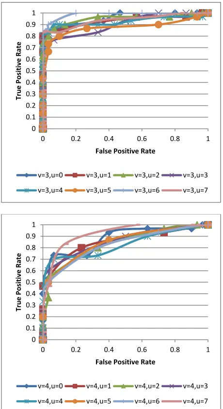
To calculate the global threshold, we used a training set of 60 subjects from our in-house dataset. Only 30 subjects were used for the gallery set. The first 30 images of the probe set were considered as the positive samples and the second 30 images as the negative samples. The face images were extracted from the first and sixth frame of the video sequence of each subjects. To find the threshold with maximum accuracy, we ran the experiment with threshold value starting from 0 to 16384, which was the highest histogram intersection value obtainable for a grayscale image with 256 bins and 64 regions. We incremented the threshold by 128. The performance of the thresholds for g , and ∑,∑ feature representations is shown in ROC curves given in Figure 8 and Figure 9 respectively. Note that in Figure 8, the ROC curves for higher scales show more discriminating thresholds which indicates the higher discriminating capability of the lower frequency filters.

When testing the chosen global thresholds calculated for the

g , and ∑,∑feature representation, we used a different set of samples for probe and gallery sets collected from second and fifth video frame, respectively. For g , feature representation, when verifying a probe image claiming to be a “positive” sample image in the gallery set, we calculated the similarity measures between them for each of the 40 filters and then compared them with their corresponding global threshold of the feature representation. If 50% or more of the similarity measures got equal or above threshold value, we accepted the probe image as a positive sample. For ∑,∑ feature representation, we checked whether the similarity measure between the probe and gallery image was above or equal to the optimal threshold chosen for authentication.

Table I provides the test results for the two feature representations.

To calculate local thresholds, a 300 image training set was used from our in-house database of 60 subjects. The training set contained 5 images each subject.

To test the local thresholds, a different set of images was used for each subject from the training set of the same subjects to create the probe and gallery set. The probe set contained a single image per subject. For the local threshold based approach, each subject was a separate class. For each class, it had 1 positive sample and 59 negative samples. Accuracy for each subject was calculated using Equation (13). We considered the performance of the g , feature representation based 40 thresholds and ∑,∑ threshold by the mean accuracy achieved on the test set.

The results of the test for both feature representations are given in Table II.

0 0.1 0.2 0.3 0.4 0.5 0.6 0.7 0.8 0.9 1

0 0.2 0.4 0.6 0.8 1

True

Positive

Rate

False Positive Rate

v=0,u=0 v=0,u=1 v=0,u=2 v=0,u=3

v=0,u=4 v=0,u=5 v=0,u=6 v=0,u=7

0 0.1 0.2 0.3 0.4 0.5 0.6 0.7 0.8 0.9 1

0 0.2 0.4 0.6 0.8 1

True

Positive

Rate

False Positive Rate

v=1,u=0 v=1,u=1 v=1,u=2 v=1,u=3

v=1,u=4 v=1,u=5 v=1,u=6 v=1,u=7

0 0.1 0.2 0.3 0.4 0.5 0.6 0.7 0.8 0.9 1

0 0.2 0.4 0.6 0.8 1

True

Positive

Rate

False Positive Rate

Figure 8. ROC curves for g , feature representation based thresholds

Figure 9. ROC curve for ∑,∑ based feature representation thresholds

Table I. Global threshold test set result for both feature representations using 60 subjects.

Filter TP FN TN FP Classification

Accuracy (%)

, 24 6 30 0 90

∑,∑ 27 3 30 0 95

Table II. Local threshold test set result for both feature representations using 60 subjects.

Feature Representation

Mean Classification Accuracy (%)

, 93.19

∑,∑ 95.89

IV. CONCLUSION

Real-time automated face verification is a challenging issue due to the variations in the data samples and time required to perform the classification objective. In this paper, we have proposed two Gabor phase feature representation based face authentication for binary and multi-class classification. Firstly, we have used the similarity measure with the highest accuracy for a Gabor feature representation as the global threshold. Secondly, we have used possible minimum threshold of individual similarity measures for each subject to classify faces. Both of these methods have shown high classification capability for our dataset with local threshold based approach showing comparably better results.

REFERENCES

[1] T. Fawcett. ROC graphs: Notes and practical considerations for researchers. ReCALL, 31(HPL-2003-4):1–38, 2004.

[2] A.J. Mansfield and J.L. Wayman. Best practices in testing and reporting performance of biometric devices. NPL Report CMSC, 14(02), 2002. [3] O.H. Jensen and R. Larsen. Implementing the Viola-Jones face detection

algorithm. Master’s thesis, Technical University of Denmark, 2008. [4] W. Zhang, S. Shan, W. Gao, X. Chen, and H. Zhang. Local Gabor binary

pattern histogram sequence (LGBPHS): A novel non-statistical model for face representation and recognition. In Tenth IEEE International Conference on Computer Vision, volume 1, pages 786–791, 2005. [5] J.G. Daugman. Two-dimensional spectral analysis of cortical receptive

field profiles. Vision research, 20(10):847–856, 1980.

[6] W. Zhang, S. Shan, L. Qing, X. Chen, and W. Gao. Are Gabor phases really useless for face recognition? Pattern Analysis & Applications, 12(3) : 301-307, 2009.

0 0.1 0.2 0.3 0.4 0.5 0.6 0.7 0.8 0.9 1

0 0.2 0.4 0.6 0.8 1

True

Positive

Rate

False Positive Rate

v=3,u=0 v=3,u=1 v=3,u=2 v=3,u=3

v=3,u=4 v=3,u=5 v=3,u=6 v=3,u=7

0 0.1 0.2 0.3 0.4 0.5 0.6 0.7 0.8 0.9 1

0 0.2 0.4 0.6 0.8 1

True

Positive

Rate

False Positive Rate

v=4,u=0 v=4,u=1 v=4,u=2 v=4,u=3

v=4,u=4 v=4,u=5 v=4,u=6 v=4,u=7

0 0.1 0.2 0.3 0.4 0.5 0.6 0.7 0.8 0.9 1

0 0.2 0.4 0.6 0.8 1

True

Positive

Rate