Online Full Text



Abstract—This work deals with the development of a finite element procedure for the steady-state and dynamic analysis of oil-lubricated cylindrical journal bearing. This procedure is employed to evaluate the applicability of simplified bearing theories, as the infinitely long journal bearing theory, that has been widely employed in the analysis and design of hydrodynamic journal bearings. Steady-state performance characteristics of hydrodynamic journal bearings are rendered by both the long journal bearing model and the finite element procedure, providing some data for a comparative analysis. The results generated by this analysis indicate that the hydrodynamic long journal bearing model must be carefully evaluated in the analysis of journal bearings because it can introduce large errors in the bearing performance predictions.

Index Terms—bearing analysis, cylindrical journal bearings, journal bearings, long bearing model

I. INTRODUCTION

The performance of industrial rotating machinery relies strongly on the efficient design of its shaft supporting bearings [1]. The technological advances on the design of fluid film bearings have given a strong impulse to the development of high performance turbomachinery [2]. Very important requirements for the fluid film bearings employed on industrial turbomachinery are not only their capability of carrying efficiently the loads generated under stringent operating conditions and providing effectively means to stabilize the rotating machine under unexpected sources of dynamic forces, but also their long operating life [3].

Lubricated journal bearings applied to industrial rotating machinery can basically be divided into two groups: fixed geometry and variable geometry bearings [4]. Of all feasible journal bearings designed for industrial rotating machinery, the fixed pad cylindrical journal bearing presents the simplest configuration and the lowest manufacturing costs [5].

The performance characteristics of cylindrical journal bearings are so important for mechanical engineering that several modern textbooks in mechanical design present technical data for their proper selection and design [6]-[8]. These technical data are generally based on the steady-state solutions for the classical Reynolds equation, which consists on the fundamental governing equation for fluid film journal

Marco Tulio C. Faria, Ph.D., is Associate Professor of the Department of Mechanical Engineering at Universidade Federal de Minas Gerais (UFMG), Av. Antonio Carlos, 6627, Belo Horizonte, MG, 31270-901, Brazil (phone: 55-31-34094925; fax: 55-31-34094823; e-mail: mtfaria@ demec.ufmg.br).

bearings [9]. Furthermore, analytical procedures based on the simplified form of the Reynolds equation have been widely used to predict the bearing behavior on the preliminary design stages [10]. Most of the practical solutions for oil-lubricated cylindrical journal bearings are based on the model of an infinite long journal bearing [10]-[11].

A pioneer work about the application of efficient finite element (FEM) procedures on the analysis of fluid film bearings is described in [12]. Since then, many efficient and accurate procedures have been devised to analyze the steady-state behavior of fluid film bearings [13]-[14]. However, the finite element prediction of the dynamic performance characteristics of oil-lubricated cylindrical journal bearings is very scarce in the technical literature [15]. The determination of the bearing steady-state performance characteristics, such as the load capacity and friction torque, and the dynamic characteristics, such as stiffness and damping force coefficients, are equally important for the development of safer, more efficient and more stable high speed rotating machinery [16].

This paper deals with a finite element procedure specially devised to analyze the static and dynamic behavior of fluid film cylindrical journal bearings. This procedure is capable of rendering both the steady-state and dynamic performance characteristics of journal bearings running under several operating conditions. The classical Reynolds equation is applied in conjunction with a linearized perturbation procedure [17] to generate the zero-th order and first order lubrication equations for the bearing, which serve to predict the bearing characteristics of interest. Firstly, the FEM procedure is used to evaluate the accuracy of the simplified theory based on the assumption of a journal bearing with infinite length or width. Secondly, predictions of the bearing dynamic force coefficients are rendered by the FEM procedure in order to provide useful technical information about the bearing dynamic behavior. Curves of bearing performance characteristics are obtained to subsidize the proper selection of the bearing configuration for rotating machinery.

II. JOURNAL BEARING PARAMETERS

Fig. 1 depicts a schematic view of a cylindrical journal bearing with its geometrical and operating parameters. The basic geometric parameters are the bearing length L and diameter D. The journal bearing rotating speed is designated by . The journal eccentricity, which is the distance between the journal center to the bearing center, can be written as e. The journal eccentricity components in the

On the Hydrodynamic Long Journal Bearing

Theory

vertical and horizontal directions are given, respectively, by

eX and eY. The dimensionless journal eccentricity ratio is defined as  = e/c, in which c represents the bearing radial clearance. The external load acting on the journal bearing is denoted by W. The bearing attitude angle, , is determined by _tan1



F_Y F_X



_{, in which FX e FY are the vertical and}

horizontal components of the bearing reaction force, respectively. The inertial reference frame is given by (X, Y,

Z) and the rotating reference frame, which is attached to the journal, is represented by (x, y, z). The journal bearing kinematics is described by using the cylindrical coordinates

R and . Hence, x = R and R is the journal radius.

Fig.1. Transverse cross-section of a cylindrical journal bearing. The thin fluid flow within the bearing clearance is described by the classical Reynolds equation. For isothermal flow of an incompressible fluid, the Reynolds equation can be expressed in cylindrical coordinates (,y,z) in the following form [5].

t ) h ( ) h ( R U 2 1 z p 12

h z p 12

h R

1 3 3

2 _

        

 

  

     

 

  

 

  

 

 

 . (1)

in the flow domain given by 02,

2 L z 2

L_{ }

 _{. The}

journal surface velocity is represented by U (U = .R). The hydrodynamic pressure, the dynamic fluid viscosity and the fluid mass density are given by p,  e , respectively. The bearing sides are at ambient pressure pa. The hydrodynamic pressure field is subjected to circumferential periodic boundary conditions, p(,z,t)=p(+2,z,t). The half Sommerfeld solution is employed in the computation of the pressure field [5]. The thin fluid film thickness h is expressed as

) ( sin ) t ( e ) cos( ) t ( e c

h  X   Y  . (2)

III. LUBRICATION EQUATIONS

The steady-state and dynamic performance characteristics of cylindrical journal bearings can be predicted by solving the zeroth and first-order lubrication equations [15]. In order to obtain these lubrication equations, a very small perturbation (eX, eY) is applied at excitation frequency () on a steady-state equilibrium position (eXo, eYo) of the journal [17]. The perturbed form for the fluid film thickness is given in the following manner.





i t

o t i Y Y X X

o e h e h e h e h e

h

h         ; (3)

Y , X



 ;i 1. (3)

where hois the steady-state or zeroth-order film thickness and hXcos(),hY sin().The small perturbations on the

fluid film thickness provoke variations on the hydrodynamic pressure field. Assuming a linear perturbation procedure, an expression for the perturbed pressure field can be written in similar form.

t i o

t i Y Y X X

o( ,t) ( e p e p )e p e p e

p ) t , (

p 

 

 _

 



      . (4)

where po and (pX, pY) represent, respectively, the zeroth-order and first-zeroth-order pressure fields. Inserting (3) and (4) into (1), the zeroth- and first-order lubrication equations can be obtained as follows.

  

 

 

 

     

 

  

     

 

  

 ( h )

R U 2 1 z p 12

h z p 12

h R

1 3 _{o o}

o o

3 o

2 . (5)

. h i ) h ( R U

z p h z p h h z p h p h h R

o o o o

o o

 

 

 

 



  

 

     

    

 

    

 

     

     

 

     



2 1

12 12

3 12

12 3

1 2 3 2 3

2

(6)

The steady-state form of the Reynolds equation (5) permits to predict the two-dimensional hydrodynamic pressure field generated by the oil film in cylindrical journal bearings. Two-dimensional industrial lubrication problems do not have closed-form solution [9]-[10]. The finite element method (FEM) has been widely employed to develop accurate procedures to solve the Reynolds equation. However, approximate analytical solutions have been often used in the analysis and design of cylindrical journal bearings [11]. These analytical solutions use simplifying assumptions based on the magnitude order of the bearing length to diameter ratio or slenderness ratio (L/D). The long bearing model, in which the axial flow is assumed very small, should provide accurate results for cylindrical journal bearings with L ≥ 2.D [18]. The validity of the one-dimensional solutions depends on the capability of determining accurately the exact value of bearing slenderness ratio that will allow predicting reliable results for a given cylindrical journal bearing and in what operating conditions these results can be used.

IV. FINITE ELEMENT MODELING

The two-dimensional thin fluid film domain is discretized by using four-node isopararemetric finite elements. The zeroth- and first-order pressure fields, given respectively by,

po e p, are interpolated over the element domain, e, through bilinear shape functions e _i1,2,3,4

i }

{



_ [19].

i i o e i e

o .p

p 



and e e_i i

e _.p

p_  _ (i = 1,2,3,4 ;  = X,Y). (7) For the finite element domain, _e_{, the Galerkin method}

equations. The zeroth-order finite element equation, which is related to the steady-state form of the Reynolds equation given by (5), can be written for a finite element e as follows.

e j e j i e o e

ji

p

f

q

k





; i,j=1,2,3,4. (8)

where e e j e i e j e i 2 3 o e

ji _{R z z} .d

1 12 h k e



















                         , e e j o e

j ₂ . d

h f e











   

 e e _{n e}

j e

j m .d

q

e





 

 . The finite element boundary is represented by e and the normal fluid flow through the border is given by

m



_n.

Similarly, the first-order finite element equation, which represents the perturbed form of the Reynolds equation given by (6), can be written as.

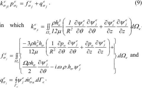
e j e j e i e

jip f q

k      . (9) (9)

in which

e e j e i e j e i 2 3 o e _d z z R 1 12 h k e ji



















   _                , e e j e j e j o e j o o

e _.d

. h . . . i h z z p p R h h f e j                                                          2 1 12 3 2 2 and e n e e j

e _{.m .d}

q

e

j _







    .

The first-order normal fluid flow through the border e of a finite element is denoted by

m



_n.

The global zeroth-order finite element equation, defined over the entire thin fluid film domain , is obtained by superposing the equations provided by (8). The solution of the zeroth-order lubrication equation leads to the steady-state hydrodynamic pressure field, which can be integrated over the fluid domain to render the bearing load capacity and other static performance characteristics, such as the friction torque and the side flow rate. The fluid film reaction forces can be estimated by the following expression, in which the ambient pressure is given by pa.

 



L _{o a}

o (p p )h R.d .dz

F 0 2 0  

  ; =X,Y. (10)

The computation of the perturbed or first-order pressure field is performed by a system of complex finite element equations obtained from (9). The numerical integration of the first-order pressure field renders an estimate for the fluid film complex impedances _{, X,Y}

o}

Z

{   . The linearized

stiffness coefficients,

{

K

_

}

_{,X,Y}, and damping coefficients,

{

C



}

_,_X,Y, associated with the fluid film

hydrodynamic action, assuming a shaft perfectly aligned, can be computed as follows.

 

  

K i C L p h R.d .dz Z 0 2 0       

 , ,X,Y. (11)

or dz . d . R . h p h p h p h p C C C C . . i K K K K L Y Y Y X X Y X X YY YX XY XX YY YX XY XX





                        0 2 0

. (12)

The synchronous dynamic force coefficients are computed at  = .

V. NUMERICAL RESULTS

For convenience, this item is divided into four sections: (a) mesh sensitivity analysis; (b) validation; (c) evaluation of the long journal bearing; (d) bearing dynamic force coefficients.

A. Mesh Sensitivity Analysis

An example of cylindrical journal bearing is selected to evaluate preliminarily the efficiency of the finite element procedure (FEM) developed in this work. Table I provides the technical data associated with this example. The curves of the journal bearing load capacity in relation to the mesh size for several eccentricity ratios is depicted by Fig. 2. The results indicate that a mesh with 800 finite elements is adequate to render reliable results for the bearing load carrying capacity. For a mesh with 800 elements, the maximum relative error found in the computation of the bearing load is about 0.3%.

TABLEI

BEARING PARAMETERS FOR MESH SENSITIVITY ANALYSIS

L = 0.012 m  = 892 kg/m3 D = 0.015 m c = 34.5x10 μm

 = 25 mPa.s Mesh size(mumber of circumferential elements multiplied by the number of axial elements)

 = 5,000 rpm

0 100 200 300

0 500 1000 1500 2000

B ea ri n g lo ad c ap ac ity (N )

[image:3.595.48.289.277.427.2]

Number of finite elements for a uniform mesh

Fig. 2. Curves of bearing load capacity versus mesh size.

B. Validation

Mechanical component design textbooks [6]-[8] usually present some curves of steady-state performance characteristics of oil-lubricated cylindrical journal bearings. A design parameter often employed to describe the bearing

e/c = 0.75 e/c = 0.5 e/c = 0.25

characteristics is the Sommerfeld number,

P N . . c R

S ₂

2



 , in

which P represents the unit load (P=W/(L.D)) and N is the journal rotation in Hz.

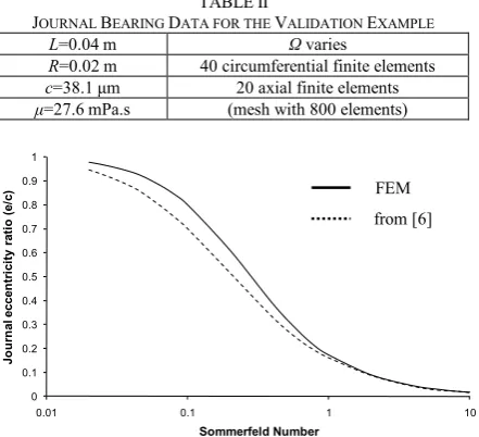
Table II shows the baseline data for the journal bearing selected for this validation example. Fig. 3 depicts the comparative results for the journal eccentricity ratio (e/c) against the Sommerfeld number for bearings with L/D=1. The solid line in this figure indicates the predictions rendered by the FEM procedure and the dashed line reproduces the results presented by the mechanical design textbooks [6[-[8]. The average relative error in this comparative analysis is about 8.5%. In many industrial applications, the Sommerfeld number is the range 1S10 [21] and the FEM predictions agree very well with the results from the classical solution of cylindrical journal bearings in this range. It is noteworthy to say that the results provided by the texbooks are based on a classical numerical work from the 1950´s [22].

TABLEII

JOURNAL BEARING DATA FOR THE VALIDATION EXAMPLE

L=0.04m Ω varies

R=0.02m 40 circumferential finite elements c=38.1μm 20 axial finite elements μ=27.6mPa.s (mesh with 800 elements)

0 0.1 0.2 0.3 0.4 0.5 0.6 0.7 0.8 0.9 1

0.01 0.1 1 10

Jo

u

rn

al

e

cc

en

tr

ic

ity

r

ati

o

(e

/c

)

[image:4.595.311.549.235.388.2]

Sommerfeld Number

Fig. 3. Comparative values of journal eccentricity ratio for cylindrical journal bearings with L/D=1.

C. Evaluation of the Long Journal Bearing Model

Table III shows the journal bearing baseline parameters employed in the evaluation of the long bearing model. In the technical literature on hydrodynamic lubrication [18] it has been stated that the infinitely long journal bearing theory is capable of generating reliable performance characteristics for bearings with L D2. This simplified theory has been widely used in hydrodynamic bearing analysis [10]-[11].

TABLEIII

BEARING PARAMETERS FOR EVALUATION OF THE LONG BEARING MODEL

L=0.03m  = 892 kg/m3 R=0.015m 60 circumferential finite elements c=34.5μm 36 axial finite elements μ=25mPa.s (mesh with 2160 elements)

Fig. 4 depicts the comparative results for the bearing dimensionless load capacity predicted by the finite element procedure (FEM) and long journal bearing theory in relation to the bearing rotating speed for slenderness ratio L/D = 2. A

more refined mesh with 2160 elements is employed in this analysis in order to ensure better numerical accuracy in the computation. The solid lines represent the FEM predictions while the dashed lines represent the values obtained from the long bearing model. The curves are shown at several eccentricity ratios. The normalization parameter for the load capacity is written as

2 3 *

c L . . . R

F    . It can be noticed that there are large discrepancies between the FEM and the long bearing theory predictions for L/D=2. Even though the long bearing theory seems to render more accurate results for lightly loaded bearings, at almost concentric operation (e=0.1), the relative deviation reaches 90% for L/D=2. The relative error increases as the eccentricity ratio increases.

0 1 2 3 4 5 6 7 8 9

1000 2000 3000 4000 5000

D

im

en

si

on

le

ss

loa

d

ca

p

acit

y

Journal rotating speed (rpm)

Fig. 4. Comparative curves of dimensionless load capacity versus rotating speed for journal bearings with L/D=2. Solid lines represent the FEM

predictions and dashed lines the long bearing model results.

Fig. 5 depicts the comparative values of dimensionless load capacity at different eccentricity ratios for journal bearings with L/D = 10. The solid lines are associated with the FEM predictions and the dashed lines with the long bearing theory results. For bearings with very light loads, the long bearing theory results agree well with the FEM predictions for longer (wider) bearings.

0 1 2 3 4 5 6 7 8 9 10

0 1000 2000 3000 4000 5000 6000

D

im

ens

io

n

les

s

lo

ad

ca

p

aci

ty

Journal rotating speed (rpm)

Fig. 5. Comparative curves of dimensionless load capacity versus rotating speed for journal bearings with L/D=10. Solid lines represent the FEM

predictions and dashed lines the long bearing model results.

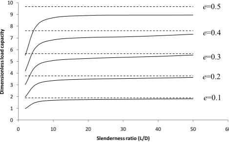
In order to show more clearly the influence of the slenderness ratio (L/D) on the long cylindrical journal bearing theory, Fig. 6 depicts some comparative curves of the dimensionless load capacity versus the slenderness ratio FEM

from [6]

e=0.1 e=0.2 e=0.3 e=0.4 e=0.5

[image:4.595.61.282.304.505.2] [image:4.595.308.544.536.685.2]

at different journal eccentricities. A constant rotating journal speed of 5000 rpm is employed to render the results shown in Fig. 6. These results demonstrate that the long bearing theory can render more accurate results for lightly loaded bearings, that is, for small eccentricity ratios. Furthermore, the slenderness ratio inferior limit L/D for the applicability of the long cylindrical journal bearing theory is well above

L/D = 2. This analysis shows that the long bearing theory can be applied to journal bearings with large slenderness ratios. The use of this simplified theory in the range

10 D L

2  must be extensively evaluated since it can render unacceptable results for the bearing performance characteristics, mainly for eccentric journal operation.

0 1 2 3 4 5 6 7 8 9 10

0 10 20 30 40 50 60

D

im

en

si

o

n

le

ss

lo

ad

ca

p

acit

y

[image:5.595.310.541.66.209.2]

Slenderness ratio (L/D)

Fig. 6. Comparative curves of dimensionless load capacity versus slenderness ratio at different journal eccentricities for Ω=5000 rpm. Solid

lines represent the FEM predictions and dashed lines the long bearing model results.

D. Bearing dynamic force coefficients

The finite element procedure developed in this work can be used to estimate some dynamic performance characteristics of fluid film journal bearings. These coefficients are crucial for the dynamic analysis of rotating shafts supported on hydrodynamic journal bearings. Table IV shows the baseline parameters associated with the journal bearing selected for this final part of the analysis. These coefficients are estimated for synchronous condition  = .

TABLEIV

BEARING PARAMETERS FOR FORCE COEFFICIENTS COMPUTATION

L=0.015m pa=101 kPa

D=0.015m 60 circumferential finite elements c=34.5μm 36 axial finite elements μ=25mPa.s (mesh with 2160 elements)

The dimensionless stiffness and damping coefficients are normalized using the following parameters.



p LD



c

K a. . /

*_{ and C}* _



_{p .L.D}



_/(c.)

a (13)

The dimensionless values of direct stiffness

K

XX and

cross-coupled stiffness KXY are graphed against the

eccentricity ratio at three journal rotating speeds in Fig. 7. The bearing becomes stiffer as the eccentricity ratio increases as well as the rotating speed increases. The same pattern is presented by the direct stiffness

K

YY and the

cross-coupled stiffness KYX as it is depicted in Fig. 8.

0 50 100 150 200 250 300

0 0.2 0.4 0.6 0.8 1

D

im

en

si

o

n

le

ss

s

ti

ffn

es

s

co

effi

ci

en

ts

K

xx

a

n

d

K

xy

[image:5.595.51.286.228.374.2]

Journal eccentricity ratio (e/c)

Fig. 7. Dimensionless stiffness coefficients K_XX(solid lines) and

XY

K (dashed lines) versus the eccentricity ratio at three journal rotating speeds.

-1000 -800 -600 -400 -200 0 200 400

0 0.2 0.4 0.6 0.8 1

D

im

en

si

o

n

le

ss

s

ti

ffn

es

s

co

effi

ci

en

ts

K

yy

a

n

d

K

yx

Journal eccentricity ratio

Fig. 8. Dimensionless stiffness coefficients K_YY (solid lines) and K_YX (dashed lines) versus the eccentricity ratio at three journal rotating speeds.

Fig. 9 depicts the curves of dimensionless direct damping coefficient

C

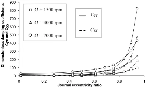
_XX and cross-coupled damping coefficient C_XY versus the journal eccentricity ratio at three journal rotating speeds. As it is expected, a raise in the journal eccentricity or in the rotating speed causes an increase in the fluid film flow viscous dissipation. At last, Fig. 10 shows the curves of the dimensionless damping coefficients CYY e CYX at the same conditions of Fig. 9.

0 500 1000 1500 2000 2500 3000

0 0.2 0.4 0.6 0.8 1

D

im

en

si

o

n

le

ss

d

am

p

in

g

c

o

effi

ci

en

ts

C

xx

e

C

xy

Journal eccentricity ratio

Fig. 9. Dimensionless damping coefficients C_XX(solid lines) and

XY

C (dashed lines) versus the eccentricity ratio at three journal rotating speeds.

e=0.1 e=0.2 e=0.3 e=0.4 e=0.5

 = 1500 rpm

 = 4000 rpm

 = 7000 rpm

KXX

KXY

 = 1500 rpm

 = 4000 rpm

 = 7000 rpm

KYY

KYX

 = 1500 rpm

 = 4000 rpm

 = 7000 rpm

CXX

[image:5.595.309.541.265.407.2]

0 100 200 300 400 500 600 700 800 900

0 0.2 0.4 0.6 0.8 1

D

im

en

si

o

n

le

ss

d

am

p

in

g

c

o

effi

ci

en

ts

C

yx

a

n

d

C

yy

[image:6.595.50.293.54.202.2]

Journal eccentricity ratio

Fig. 10. Dimensionless damping coefficients C_YY(solid lines) and

YX

C (dashed lines) versus the eccentricity ratio at three journal rotating speeds.

VI. CONCLUSIONS

Two important conclusions can be drawn from the analysis presented in this work. Firstly, the range of applicability of simplified journal bearing theories must be carefully evaluated prior to their application. The inferior limit of the bearing slenderness ratio range that make the long bearing theory acceptable from the accuracy standpoint can be very different from the value L/D=2 found in the vast technical literature about fluid film journal bearings. Secondly, the accurate analysis of oil lubricated cylindrical journal bearings requires the development of efficient numerical procedures. Industrial journal bearings usually present slenderness ratio in the range 0.5L/D1, in which the simplified bearing theories are not capable of rendering accurate predictions for the bearing performance characteristics.

REFERENCES

[1] F.Y. Zeidan and B.S. Herbage,”Fluid film bearing fundamentals and failure analysis,” in Proc. 20th _{Turbomachinery Symposium, Houston,}

1991, pp. 161-186.

[2] F.Y. Zeidan,”Developments in fluid film bearing technology,” Turbomachinery International, September/October 1992, pp. 1-8. [3] K. Knöss, “Journal bearing for industrial turbosets”, Brown Boveri

Review, vol. 67, 1980, pp. 300-308.

[4] P.E. Allaire and R.D. Flack, “Design of journal bearings for rotating machinery,” in Proc 10th _{Turbomachinery Symposium, Houston,}

1981, pp. 25–45.

[5] B.J. Hamrock, Fundamentals of Fluid Film Lubrication. New York: McGraw-Hill, 1994.

[6] R.C. Juvinall and K.M. Marshek, Fundamentals of Machine Component Design. New York: John Wiley & Sons, 5th _{Ed., 2012.} [7] R.G. Budynas and J.K. Nisbett, Shigley´s Mechanical Engineering

Design. New York: McGraw-Hill, 9th _{Ed., 2011.}

[8] R. Norton, Machine Design – An Integrated Approach. New York: Prentice-Hall, 2nd _{Ed., 2000.}

[9] A.Z. Szeri, Tribology: Friction, Lubrication and Wear. New York: McGraw-Hill, 1980.

[10] L. San Andrés,”Approximate design of statically loaded cylindrical journal bearings,” ASME Journal of Tribology, vol. 111, pp.390-393, 1989.

[11] D.C. Sun,”Equations used in hydrodynamic lubrication,” STLE Lubrication Engineering, vol. 53, 1997, pp.18-25.

[12] M.M. Reddi, “Finite element solution of incompressible lubrication problem”,” ASME Journal of Lubrication Technology, vol. 91 , 1969, pp. 524-533.

[13] J.F. Booker and K.H. Huebner,”Application of finite element methods to lubrication: an engineering approach,” ASME Journal of Lubrication Technology, vol. 94, 1972, pp.313-323.

[14] P. Allaire, J. Nicholas, and E. Gunter,”Systems of finite elements for finite bearings,” ASME Journal of Lubrication Technology, vol. 99, 1977, pp.187-197.

[15] M.T.C. Faria, F.A.G. Correia, and N.S. Teixeira,”Oil lubricated cylindrical journal bearing analysis using the finite element method,”in Proc. 19th _{International Congress of Mechanical}

Engineering, Brasília, Brazil. 2007, pp.1-10.

[16] D.W. Childs, Turbomachinery Rotordynamics: Phenomena, Modeling & Analysis. New York: McGraw-Hill, 1993.

[17] P. Klit and J.W. Lund,”Calculation of the dynamic coefficients of a journal bearing, using a variational approach,” ASME Journal of Tribology, vol. 108, 1986, pp.421-425.

[18] A.Z. Szeri,”Some extensions of the lubrication theory of Osborne Reynolds,” ASME Journal of Tribology, vol.109, 1987, pp.21-36. [19] K.J. Bathe, Finite Element Procedures in Engineering Analysis.

Englewood Cliffs, NJ: Prentice-Hall, 1982.

[20] K.H. Huebner, E.A. Thornton, and T.G. Byrom, The Finite Element Method for Engineers. New York: John Wiley & Sons, 1995. [21] F.A.G. Correia, “Determinação das características de desempenho de

mancais radiais elípticos utilizando o método de elementos finitos”, M.Sc. Thesis, Graduate Program in Mechanical Engineering, Universidade Federal de Minas Gerais, Belo Horizonte, Brazil, 2007. [22] A.A. Raimondi and J. Boyd,”A solution for the finite element journal

bearings and its application to analysis and design – I, II, and III,” ASLE Transactions, vol. 1, 1958, pp. 159-209.

 = 1500 rpm

 = 4000 rpm

 = 7000 rpm

CYY