Published in: J. Mater. Sci., vol. 37, 2002, 287-294
MOISTURE UPTAKE IN MONOLITHIC AND COMPOSITE MATERIALS:
EDGE CORRECTION FOR RECTANGULOID SAMPLESM.J. Starink, L.M.P. Starink* and A.R. Chambers
Materials Research Group, School of Engineering Sciences, University of Southampton, Southampton SO17 1BJ, UK
*currently at QinetiQ, Farnborough GU14 OLX, UK Abstract
Experiments on moisture uptake of monolithic and composite materials are generally performed by immersing rectanguloid (square plate) samples in water. An edge correction factor is derived which, in a mathematically simple way, takes water uptake through all 6 faces (2 broad and 4 smaller faces) into account. Analysis shows this edge correction factor to be very accurate (deviations typically less than 2%). New expressions for moisture uptake in composites with unidirectionally aligned fibres are derived, by incorporating this edge correction factor as well as proper boundary conditions which depend on volume fraction of fibres. Experimental data on moisture uptake in these types of composite samples is successfully analysed using these expressions.
1. Introduction
In the present publication it will be shown that Shen and Springer’s edge correction factor is inaccurate and in section 2.2 a new accurate edge correction factor will be derived. The new edge correction factor will be used to obtain expressions for the moisture uptake composites with unidirectional fibres (section 2.3). The latter expressions will be used to analyse data on the moisture uptake in composites with unidirectional fibres (section 3).
2 Mathematical treatment of diffusion in monolithic and composite materials 2.1 1D and 3D Fickian diffusion
If moisture uptake is determined by classical 1D Fickian diffusion, the moisture concentration as a function of time, t, and distance from the surface, x, is given by the well known solution for diffusion in an infinite plate (see for instance Refs. [4,5,6]):
(
)
c x t c
c c j
j x
a
j D t
a
i
m i j
x
( , )
( ) sin( ) exp
−
− = − +
+
− +
⎡
⎣ ⎢ ⎢
⎤
⎦ ⎥ ⎥ −
= ∞
∑
1 4 2 1 2 2 1 2 1
0
2 2 2 π
π π
(1)
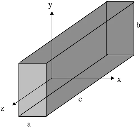
where c(x,t) is the moisture concentration, ci is the initial moisture concentration (assumed to be uniform), cm is the maximum moisture concentration, Dx is the diffusivity in the x direction (the direction normal to the broad faces) and a is the thickness of the sample in the x direction.
z
y
x
a
b
c
Fig. 1 Orientation of rectanguloid with respect to the axes.
[image:2.595.176.412.445.662.2](
)
M =G Mm−Mi +Mi (2)
where Mi is the initial moisture content, Mm is the maximum moisture content, and
(
)
(
)
G G j j D t
a D j x = = − + ⎡− + ⎣ ⎢ ⎢ ⎤ ⎦ ⎥ ⎥ − = ∞
∑
1 2 2 0 2 2 21 8 2 1 2 1
π
π
exp (3)
For G <0.6 the above equation can be approximated very accurately by:
π t D a G x D 4
1 ≅ (4)
Hence the moisture uptake is a linear function of t1/2 and the diffusion coefficient Dx can be obtained directly from the initial slope of a plot of (M-Mi)/(Mm-Mi) vs. t1/2/a, using:
slope≅4 Dx
π (5)
For samples of finite dimensions Eq. 4 is only a rough approximation and in order to make accurate determinations of the diffusion constant, and to be able to compare samples of different shapes, the uptake through the smaller faces needs to be taken into account. One could of course resort to the solution for the full three dimensional problem of diffusion in a rectanguloid (ie. a rectanguloid) [2,4]:
(
)
(
)
(
)
(
) (
) (
)
G t k a D l b D m c Dk l m
D
k l m
x y z
3 2
3
0 0 0
2 2 2 2 2 2 2
2 2 2
1 8
2 1 2 1 2 1
2 1 2 1 2 1
= −⎛ ⎝⎜ ⎞ ⎠⎟ − ⎛ + + + + + ⎝ ⎜⎜ ⎞⎠⎟⎟ ⎡ ⎣ ⎢ ⎢ ⎤ ⎦ ⎥ ⎥ + + + = ∞ = ∞ = ∞
∑ ∑ ∑
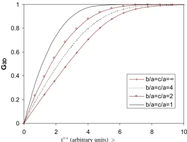
π π exp (6) where k, l and m are positive whole integers, Dx, Dy and Dz are the diffusion coefficients in the direction of the 3 axes, and a, b and c are the sides of the rectangular parallelepiped (or rectanguloid) the x, y and z directions. (See Fig. 1, we will take a ≤ b ≤ c.) In monolithic materials Dx, Dy and Dz will, in general, be equal. For a << b,c and G3D < 0.6 a plot of G3D vs.t1/2/a is again in good approximation linear (see Fig. 2 and Ref. [2]). In analogy to the 1D diffusion case we can thus define an effective apparent diffusion coefficient, Deff, by:
slope
Deff
t1/2 (arbitrary units) >
Fig. 2 Total normalised moisture uptake in a rectanguloid (G3D) as a function of t1/2.
2.2 Edge correction factors for monolithic rectanguloids
Eq. 6 can only be evaluated at the expense of much more computer time than is needed for evaluation of Eq. 1. A more important drawback of Eq. 6 is that although for a << b,c and G3D < 0.6 a plot of G vs. t1/2 is again approximately linear [2], a method for calculation of the diffusion constant from the slope of such a plot is not easily determined. For this reason it is very useful to derive a correction factor, f, that takes the influence of diffusion through the smaller faces into account such that:
G3D = f G1D(G3D < 0.6) (8)
and hence,
Dc= f--2Deff (9)
Where Dc is the diffusion constant estimated from moisture uptake data for in a rectangular paralellepiped corrected using factor f. Shen and Springer [1] have in the past claimed to have derived just such a correction factor. For D = Dx = Dy = Dz Shen and Springer’s edge correction factor is given as:
0 0.2 0.4 0.6 0.8 1
0 2 4 6 8 10
G
3Df f a b
a c
S S
≈ & = + +1 (10)
However, as will be shown below, Shen and Springer’s edge correction factor is inaccurate and overestimates f by a considerable amount. In the following we will show that a much more accurate edge correction factor can be derived.
For the derivation of the edge correction factor we will consider a rectanguloid solid of dimensions a, b, c (a ≤ b ≤ c) which is exposed to a constant humidity environment.
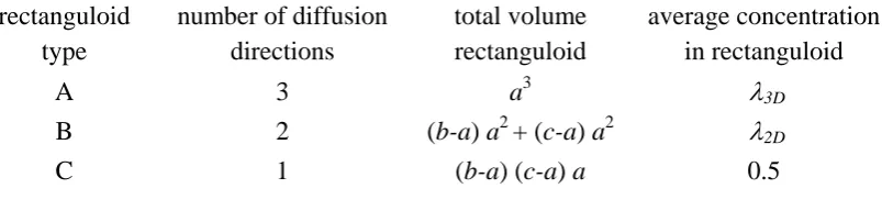
Fig. 3 Rectanguloid divided into 3 types of different sub-rectanguloids.
Table 1 Properties of rectanguloids in Fig. 3. rectanguloid
type
number of diffusion directions
total volume rectanguloid
average concentration in rectanguloid
A 3 a3 λ3D
B 2 (b-a) a2 + (c-a) a2 λ2D
C 1 (b-a) (c-a) a 0.5
In order to derive the general mathematical form that f will take we will first consider an approximate treatment. In this first approximate treatment we will make the following simplifying assumptions:
i) the concentration at any given point in the solid is determined solely by the time and the distance to the nearest external surface.
ii)the concentration drops linearly with distance to the nearest surface.
Consider the time, tx, at which the moisture has just reached all parts of the solid, i.e. the time at which the moisture just reaches the point(s) furthest away from the surfaces. To calculate
C
B A
a/2 a/2
b-a
[image:5.595.118.441.258.392.2] [image:5.595.79.481.497.598.2]the average moisture content it is convenient to subdivide the solid into three types of rectanguloids according to the number of directions from which diffusion has occurred into these rectanguloids. For instance (see Fig. 3), on all 8 corners of the solid, cubes of side ½a are found in which the concentration profile is determined by diffusion from three mutually perpendicular directions. Connecting pairs of these cubes along the four smaller faces of the solid are rectanguloids in which the diffusion profile is determined by diffusion from two directions. In the remainder of the solid, the diffusion profile is determined by diffusion perpendicular to the broad faces only. Properties of the three types of rectanguloids (termed A, B and C, respectively) are listed in Table 1.
The average concentration in rectanguloids of each type is constant and can be calculated through integration. From the data in table 1 the average concentration in the solid, C, equals:
[
]
C a a b a c a a b a c a
a b c
D D
= + − + − + − −
3
3 2 2 12
λ ( ) ( ) λ ( )( )
(11)
If the diffusion had only occurred through the two broad faces the average concentration would have been ½ , hence it follows that,
(
)
[
]
(
)
f C a b a c a
bc
a bc
D D
= = + − − + − + −
½ 1 2 2 2
1
2 3 12
2
λ ( ) ( ) λ (12)
which simplifies to:
bc a c a b a fSSC
2
2 1 1
1+λ +λ +λ
= (13)
where λ1 and λ2 are functions of λ2D and λ3D. There are several ways in which λ1 and λ2 (or λ2D and λ3D) can be derived*, the most accurate analysis being obtained by fitting their values using the complete 3D diffusion equation and calculating the slope of the initial part. Thus, in the next stage of the analysis, average moisture uptake as a function of t was calculated with Eq. 6 for various shapes of rectanguloids, using D = Dx = Dy = Dz. From these profiles Deff and Dc were obtained from the slope of a plot of G vs. t1/2 (G from 0 to 0.5) for:
i) f = 1 (i.e. assuming one dimensional diffusion only), ii) f = fS&S (Shen and Springer's edge correction),
iii) f = fSSC (our edge correction factor, Eq. 13), with optimised values for λ1 and λ2. It was found that for Eq. 13 the best results were obtained for λ1 = 0.54, λ2 = 0.33. Hence Eq 13 becomes:
*
Using assumptions i) and ii) one finds λ1= 1
/3 and λ2= 1
/6. Analysis of the accuracy of this
bc a c
a b
a fSSC
2
33 . 0 54 . 0 54 . 0
1+ + +
= (14)
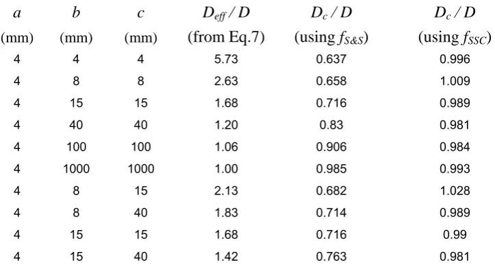
Final results are presented in Table 2, which shows:
a) fS&S (Shen and Springer's edge correction) is quite inaccurate and it considerably over corrects for the edge effect for all sample shapes. For realistic sample shapes deviations in D are between 16 and 37%.
b) Eq. 13 gives an accurate approximation for the edge effect. Deviations in D are typically less than 2%.
[image:7.595.77.439.382.585.2]Thus, in concluding this section, in analysis of moisture uptake data for a finite monolithic sample the diffusion coefficient can be obtained from the initial slope (from G = 0 to 0.5) of a sorption curve via Eq. 5, where the edge correction factor f is given by Eq. 14.
Table 2 Dc calculated by applying edge correction factors derived by Shen and Springer (fS&S) and by the present authors (fSSC).
a
(mm)
b
(mm)
c
(mm)
Deff / D (from Eq.7)
Dc / D (using fS&S)
Dc / D (using fSSC)
4 4 4 5.73 0.637 0.996
4 8 8 2.63 0.658 1.009
4 15 15 1.68 0.716 0.989
4 40 40 1.20 0.83 0.981
4 100 100 1.06 0.906 0.984
4 1000 1000 1.00 0.985 0.993
4 8 15 2.13 0.682 1.028
4 8 40 1.83 0.714 0.989
4 15 15 1.68 0.716 0.99
4 15 40 1.42 0.763 0.981
2.3 Diffusion in unidirectional composites
In unidirectional composites the diffusion rates can, in general, be expected to be direction dependent. Several authors [1,2] presented a mathematical treatment of this, but an overhaul of this work has become necessary because:
1. In earlier work [1,2] Shen and Springer’s inaccurate edge correction factor, fS&S, was used. 2. Most expressions used in Refs. [1,2] for diffusion in composites are only valid for steady
state conditions. The limitations for water uptake were not assessed in Refs. [1,2].
A modified treatment of diffusion in unidirectional composites is presented below.
In a unidirectional composite containing cylindrical fibres, the thermal conductivity of the composite normal to the fibres, K⊥, can be measured by taking a large thin plate and imposing two temperatures T1 and T2 on the two broad faces. In steady state conditions, K⊥ is in good approximation given by (see Ref. [1]):
K
v
K K
B B v
B v
B v
f r
r
k k f
k f k f ⊥ ≅ − − ⎛ ⎝ ⎜ ⎜ ⎞ ⎠ ⎟ ⎟ + − − − + ⎡ ⎣ ⎢ ⎢ ⎤ ⎦ ⎥ ⎥
1 2 4
1 1 1 2 1 2 2
π π π
π π
tan (15)
B K K k r f = ⎛ − ⎝ ⎜⎜ ⎞⎠⎟⎟
2 1 (16)
where vf is the volume fraction of fibres, Kr is the thermal diffusivity in the resin/matrix, and
Kf is the thermal diffusivity in the fibres. As heat conduction in solids and diffusion are equivalent in mathematical terms (see e.g. Ref. [4]) it follows that, under equivalent boundary conditions, the diffusivity in the composite normal to the fibres, D⊥, is in good approximation
given by:
D
v
D D
B B v
B v
B v
f r
r
D D f
D f D f ⊥ ≅ − − ⎛ ⎝ ⎜ ⎜ ⎞ ⎠ ⎟ ⎟ + − − − + ⎡ ⎣ ⎢ ⎢ ⎤ ⎦ ⎥ ⎥
1 2 4
1 1 1 2 1 2 2
π π π
π π
tan (17)
B D D D r f = ⎛ − ⎝ ⎜⎜ ⎞⎠⎟⎟
2 1 (18)
where Dr is the thermal diffusivity in the resin/matrix, and Df is the thermal diffusivity in the fibres.
In the steady state, the diffusivity in the composite parallel to the fibres, D//, is simply given
by:
D/ / = −(1 vf )Dr +v Df f (19)
It is important to note that the above equations are only valid provided:
1. Diffusion (heat conduction) occurs under steady state conditions i.e. local moisture concentration c(x,y,z) (temperature T(x,y,z)) is independent of time.
2. Boundary conditions imposed are constant and independent of vf.
As an illustration of complexities encountered in composites we consider the case where Df <<
Dr and both the saturation levels in resin and fibre, Mm,r and Mm,f are significant. In this case diffusion of moisture will initially occur only in the matrix and only after the matrix has taken up a substantial amount of water the fibres will take up significant amounts of water, essentially acting as a sink for moisture within the matrix. Thus, steady state can only be reached a long time after substantial diffusion through the matrix has occurred. In such a case moisture uptake is a two stage process and solutions can not be derived on the basis of a single stage 3D diffusion equation (or a 1D equation with edge correction) with appropriate insertion of expressions for D⊥ and D//†.
In general terms, the above equations can yield solutions or partial solutions for moisture uptake in the following cases:
A.Mm,f << Mm,r. In this case moisture entering the fibre is insignificant. A complete solution can be obtained.
B.Df= 0. No moisture enters the fibre. A complete solution can be obtained.
C. a Dr >> d Df (d is the fibre diameter) Moisture uptake in the fibre becomes significant only in a second stage after the resin has saturated. A solution for the first stage can be obtained.
In the following we will obtain solutions for cases A, B, and the first stage of C.
In obtaining the solutions for the above cases we first need to obtain the appropriate boundary condition. As at each outer surface of the composite contains a fraction vfof fibre ends which do not absorb water, the average boundary condition at the outer surfaces is given by:
c surface( )= −(1 vf )Mr m, (20)
(Note that this is different from the steady state heat conduction composites for which the surface temperature equals the environment temperature, i.e. the boundary condition is independent of vf.) The volume averaged diffusivities parallel and normal to the fibres can now be obtained in the following manner. As no water is taken up by the fibre, the diffusivity in the direction parallel to the fibres is simply given by:
D/ / = Dr (21)
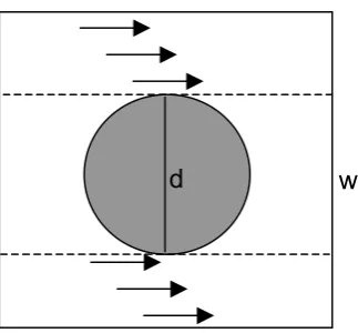
Average diffusivity normal to the fibres can be analysed using the simplified geometry of blocking of flow in a square packing array depicted in Fig. 4. Using Fick’s first law:
x c D F
Δ Δ −
= (22)
it follows:
†
d w
Fig. 4 Simplified geometry for diffusion normal to fibres in a square packing array.
[
]
11
1 −
⊥ ⎟ −
⎠ ⎞ ⎜ ⎝ ⎛ −
= r vf
w d D
D (23)
where d is the diameter of the fibre and w is the width of the square. In this equation the term [1-vf]-1 reflects the change in boundary condition (average surface concentration) resulting from the introduction of the impermeable fibres. (This term does not appear in the case of steady state heat conduction in a composite and was not accounted for in Refs. [1,2].) From the latter equation it follows:
r f
f
D v
v
D
− ⎟ ⎟ ⎠ ⎞ ⎜
⎜ ⎝ ⎛
− =
⊥
1 2 1
π
(24)
If the fibres are oriented relative to the axes in the manner presented in Fig. 5 then the diffusion coefficients in the different directions are given by:
Dx =D/ / cos2α+D⊥ sin2α (25)
Dy = D/ / cos2β+D⊥ sin2 β (26)
Dz = D/ / cos2γ +D⊥ sin2γ (27)
β
α
γ
x
y
z
Fig. 5 Orientation of fibres with respect to the axes.
From Eq. 6 it follows that the edge correction factor for materials in which Dx ≠ Dy ≠ Dz can be derived simply by substituting a Dx , b Dy and c Dz for a, b and c in the corresponding equations. Thus an accurate edge correction factor for materials with direction dependent diffusivity is:
f a
b D
D
a c
D D
a bc
D D
D
y
x
z
x
z y
x
= +1 1 + 1 + 2
2
2
λ λ λ (28)
(Note that in substituting a Dx , b Dy and c Dz for a, b and c, the axes are chosen such that a Dx ≤ b Dy ≤ c Dz . Hence a is no longer necessarily the shortest edge of the rectanguloid.)‡ Hence for G < 0.6 the moisture uptake can be obtained from:
G f a
Dt
≅ 4 π (29)
Thus for G < 0.6 the moisture uptake can be approximated accurately, using Eq. 21 and 24-27 combined with Eq. 2. As a specific examples we will consider the cases of rectanguloids with fibres parallel to one of the axes of the sample.
‡
Similarly, Shen and Springer’s edge correction factor for materials with direction dependent diffusivity becomes:
f a
b D
D a c
D D
S S
y
x
z
x
Case 1: Df = 0 and α = 0
As the fibres are parallel to the x-axis (i.e. α = 0):
Dx =D// (30)
Dy = Dz =D⊥ (31)
The moisture uptake in the initial part (G < 0.6) can be obtained by using:
D D a
b a c v v eff r f f
(α ) λ
π = ≅ + ⎛⎝⎜ + ⎞⎠⎟ − − ⎡ ⎣ ⎢ ⎢ ⎤ ⎦ ⎥ ⎥ 0 1 1 2 1 1 2 (32)
(here second order edge effects are neglected by taking λ2 = 0). The saturation level in the composite is given by:
Mm c, ≅ (1−vf )Mm r, (33)
Case 2: Df= 0 and β = 0
In a similar fashion one obtains:
D D v v a b v v a c eff r f f f f
(β )
π λ π = ≅ − − + − − + ⎛ ⎝ ⎜ ⎜ ⎞ ⎠ ⎟ ⎟ ⎡ ⎣ ⎢ ⎢ ⎤ ⎦ ⎥ ⎥ 0 1 2 1 1 1 1 2 1 2 (34)
The saturation level is given by Eq. 33. Case 3: Df = 0 and γ = 0
This is obtained by exchanging b and c from the previous equation:
D D v v a b a c v v eff r f f f f
(γ )
π λ π = ≅ − − + + − − ⎛ ⎝ ⎜ ⎜ ⎞ ⎠ ⎟ ⎟ ⎡ ⎣ ⎢ ⎢ ⎤ ⎦ ⎥ ⎥ 0 1 2 1 1 1 1 2 1 2 (35)
The saturation level is given by Eq. 33.
3 Experimental
In order to validate the expressions derived in the previous section, moisture absorption experiments were performed on sections cut from a single 1.6 mm thick panel with cylindrical fibres unidirectionally aligned parallel to the surface (for full details see Ref. [7]) as well as on sections from a corresponding unreinforced resin panel. The resin system in both cases was epoxy blended with 30wt% of thermoplastic (PES). The unreinforced panel was produced at ICI Wilton, using a standard technique for production of neat resin plaques. The thermoplastic was dissolved in a solvent and then added to the epoxy and hardener. The solvent was then evaporated off. Next, each blend was cast into an open mould, preheated to 413K, and degassed for 30 min under vacuum to remove residual solvent and trapped air. Samples were then cured at 458K for 120 min and allowed to cool to room temperature for a further 120 min. The reinforced panels (also produced at produced at ICI Wilton) were manufactured using unidirectional carbon tape, which was pre-impregnated with the 30% thermoplastic resin before lay-up. The panel was made to be approximately 1.6 mm thick, and 130 mm square. The cure was carried out in a pressclave using edge dams to ensure maximum flow through the panel thickness, to minimise voidage. The cure cycle involved a heating ramp to 458K over 80 min, a dwell at 458 K for 180 min and a ramp down to room temperature over 80 min. From the saturation levels of the composites and the corresponding unreinforced matrix the fibre content was calculated as 74 vol% (using Eq. 33). Optical microscopy on cross sections of the samples (see Ref. [7]) confirmed that porosity in the samples was low and that the fibres in the reinforced panel were generally well aligned.
The reinforced panel was cut into rectanguloid samples of varying shape ranging from 1.6 × 10 × 100 mm to 1.6 × 100 × 10 mm and 1.6 × 60 × 60 to 1.6 × 10 × 10 mm (a × b ×c), see Table 3, with fibres aligned in the b direction. For some of the sample types duplicate experiments were employed, i.e. two nominally identical samples cut from the same panel and with identical dimensions and identical direction of fibres, were exposed in the same bath at the same time. The samples were totally immersed in water at 25ºC and for all samples the initial part of the curve of (M-Mi)/(Mm-Mi) vs. t1/2 was in good approximation a straight line.
Mm was assumed to be identical for all samples and Deff was calculated from the slope.
4 Results and discussion
It should be noted that thoughout the present analysis we will assume that the fibres do not absorb moisture. It is believed that this is a good approximation for the carbon fibres.
an anomalously high value of Deff/Dr was ascribed to a flawed section of the panel and omitted from the analysis.)
To analyse the data, first the theoretical predictions for Deff/Dr were calculated using Eqs. 32 and 34 (using λ1 = 0.54, according to our edge correction factor). This data was used to obtain
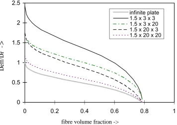
Dr through fitting to the experimental data and in Fig. 7 the resulting experimental Deff/Dr values are compared with the theoretical predictions. Fig. 7 shows a good correspondence between experimental and measured Deff/Dr (χ2 is 1.0) proving that Eqs. 32 and 34 (which incorporate our new edge correction factor) are sound. Conversely, employing Shen and Springer’s edge correction factor (i.e. Eqs. 32 and 34 with λ1 = 1) yields a much worse correspondence (χ2 is about 6).
For a final comparison of the model predictions with the data the ratio of the diffusion coefficients of the 1.6 × 100 × 10 mm composite panel to that of the unreinforced panel was calculated from the experimental data. This yields 0.11, which is in reasonable agreement with the results presented in Fig. 7. Thus, it is concluded that the present analysis leading to Eqs. 34 and 35 can explain all observations of the relative water uptake rates of the present unidirectionally reinforced panels and the unreinforced panel.
0 0.5 1 1.5 2 2.5
0 0.2 0.4 0.6 0.8 1
infinite plate 1.5 x 3 x 3 1.5 x 3 x 20 1.5 x 20 x 3 1.5 x 20 x 20
[image:14.595.119.476.409.660.2]fibre volume fraction ->
Fig. 7 Deff/Dr for unidirectional composite rectanguloids of different shapes.
Table 3 Dimensions of rectanguloid shaped composites used for moisture uptake experiments. Fibres are aligned along the y-axis (i.e. parallel to edge of length b).
type a
(mm) b (mm)
c (mm)
A 1.6 10 120
B 1.5 120 10
C 1.6 20 60
D 1.5 60 20
E 1.5 30 40
F 1.6 10 10
G 1.6 20 20
H 1.6 40 40
I 1.5 60 60
4 Concluding remarks
The analysis of edge effects in section 2.2 has shown that Shen and Springer’s edge correction factor, fS&S (Eq. 10), is inaccurate and analysis of experiments as presented in section 3 further confirmed this result. As fS&S has in the past been used in many analyses of experimental data of moisture uptake D values obtained in these works should in general be corrected by
0 0.05 0.1 0.15 0.2 0.25
10x120 120x10 20x60 60x20 30x40 10x10 20x20 40x40 60x60 inf. plate
Deff/Dr ->
[image:15.595.82.256.449.644.2]multiplying with (fS&S/fSSC)2. The magnitude of this correction is in the order of 15 to 30% for typical sample dimensions. It is further noted that also for disc shaped samples correction for edge effects is necessary. With the concepts presented in section 2.2, in principle, edge correction factors for discs and other types of regular shapes can be derived.
The treatment presented in section 2.3 shows that introduction of fibres that take up little or no water reduces the rate of water uptake in two ways:
1. the maximum moisture uptake is reduced
2. the diffusion rate of water in a direction perpendicular to the fibres is reduced.
Thus whilst the reduction of maximum moisture uptake is independent of fibre orientation the diffusion rate of water is strongly influenced by the way in which the fibres are oriented. As an example Fig. 7 shows that for an infinitely large plate Deff/Dr = 0.11, i.e. the introduction of 0.74vol% of cylindrical fibres both decreases the maximum water uptake to 26% of that of the unreinforced resin and decreases the absorption rate by a factor 0.11, provided the plate is flawless and has a homogeneous distribution of fibres. Local variations of density of fibres and other flaws which yield high diffusivity paths perpendicular to the fibres can significantly increase the rate of moisture uptake in unidirectional panels.
References
1 C.H. SHEN and G.S. SPRINGER, J. Comp. Mater.10 (1976) 2
2 M. T. ARONHIME, S. NEUMANN and G. MAROM, J. Mater. Sci. 22 (1987) 2435 3 M.E.R. SHANAHAN and Y. AURIAC, Polymer39 (1998) 1155
4 H.G. CARSLAW and J.C. JAEGER, in “The Conduction of Heat in Solids”, 2nd ed (Oxford University Press, London, 1959)
5 J. CRANK, in “ The Mathematics of Diffusion”, 2nd ed. (Oxford University Press, London, 1975)