Invariant Characterization of the Hough Transform for Pose Estimation of Arbitrary Shapes

On Resolving Ambiguities in

Arbitrary-Shape extraction by the

Hough Transform

Eugenia Montiel

, Alberto S. Aguado

and Mark S. Nixon

iMAGIS, INRIA Rhône-Alpes, France

University of Surrey, UK

University of Southampton, UK

Abstract

The Hough transform extracts a shape by gathering evidence obtained by mapping points from the image space into a parameter space. In this process, wrong evidence is generated from image points that do not correspond to the model shape. In this paper, we show that significant wrong evidence can be generated when the Hough Transform is used to extract arbitrary shapes under rigid transformations. In order to reduce the wrong evidence, we consider two types of constraints. First, we define constraints by considering invariant features. Secondly, we consider constraints defined via a gradient direction information. Our results show that these constraints can significantly improve the gathering strategy, leading to identification of the correct parameters. The presented formulation is valid for any rigid transformations represented by affine mappings.

1

Introduction

The Hough Transform (HT) gathers evidence for the parameters of the equation that defines a shape, by mapping image points into the space defined by the parameters of the curve [1,2]. After gathering evidence, shapes are extracted by finding local maxima in the parameter space (i.e., local peaks). In a broad definition, the HT can be generalized to extract arbitrary models by changing the equation of the curve under detection [1]. For general forms, the curve under detection can be defined by combining the equation of a shape and a parameterized transformation [3]. Thus, the parameters of the model are actually the parameters of the transformation that represents the different appearances of a shape in an image. Most general forms of the HT has been defined for similarity transformations [4,5], although recently there has been an interest on affine and more general mappings [6,7].

that the analysis of clustering techniques and hypothesis strategies of clustering techniques can be used to establish the performance of the generalized forms of the HT, the difference in the type of features used by both techniques makes the uncertainty under occlusion and noise essentially different [13]. Since geometric hashing is based on primitives such as lines, curves or polygons, then the range of evidence accumulated is increased by small errors in the primitives. Conversely, the HT and its generalizations gather evidence by using single points. Thus, performance depends on random matching, rather than on errors in the computation of image primitives.

In this paper, we show that significant wrong evidence can be generated when the HT is used to extract arbitrary shapes under rigid transformations. The importance of false evidence is directly related to the generality in which the HT is defined. Intuitively, as the transformation that defines the appearance of a model shape becomes more general, then local image information is less significant. Thus, image features can easily produce false evidence. That is, as the transformation becomes more general, the model increases the number of possible forms to be matched. Therefore, the model can easily be matched to noise or to segments of objects that do not correspond to the description of the whole shape. The false evidence generated can interfere seriously with the detection process causing inaccurate, or even incorrect, results.

Here, we study the significance of wrong evidence for arbitrary shapes under affine transformations. In this case, the generality of the transformation can produce an excessive amount of wrong evidence that can spoil the extraction process. In order to ameliorate this problem, we use two types of constraints. First, we define constraints by considering invariant features. Secondly, we consider constraints defined via a gradient direction information. Constraints are used to verify whether the transformation is congruent to the image information. Our results show that these constraints can significantly improve the gathering strategy of the HT. The presented formulation is valid for general geometric transformations, however, our examples and results are developed for affine transformations only.

This paper is organised as follows. For completeness, section 2 presents the definition of the HT for arbitrary shapes. Arbitrary shapes are parameterised by continuous curve under rigid transformations represented by affine mappings. In section 3 we discuss the source of wrong evidence in the HT. Notice that this is different to the combinatorial error discussed in [8]. In the HT wrong evidence is generated when the model is matched against false evidence independently of the accuracy in the data. In section 4 we consider constraints to reduce false evidence during the gathering process. Section 5 presents implementations and examples. Section 6 includes conclusions.

2

General shapes and affine mappings

2.1

HT mapping

The HT gathers evidence of a model shape through a mapping defined between the image space and the parameter space. In this section, we are interested in obtaining a formal representation of this mapping when the model is given by an arbitrary shape under an affine mapping.

parameters of the transformation become the parameters of the model. In order to exemplify these concepts we can consider a circle with radius one and centred on the origin to be a shape without any parameters. If we apply an affine transformation to the shape, then the model is given by an ellipse. Each of the five parameters of the ellipse is related to the parameters of the affine transformation. Thus, when we find an ellipse in an image, we are actually finding a transformed circle. It is important to notice that in this approach the complexity of the extraction process is independent of the complexity of the shape. That is, if we replace the circle by a complex shape such as the profile of a mountain or the course of a river, then the model defining its appearance will still have five parameters. Therefore, the HT mapping for the circle and the complex shapes both have a five-dimensional accumulator space and the extraction process involves the same complexity.

If we consider an arbitrary shape given by the curve υ( ), then a parametric model is composed of the points,

(ab ) f( )a b

w , ,υ = ,υ + , (1)

for υ ∈υ( )s a point in the shape. The parameters of the transformation have been divided into the translation and the deformation parameters. If we consider an image point p, then we can match this point to a point in the model. This would imply that

(a, b,υ)

w

p= . Thus, by solving for b in equation (1), we have that

(p,υ,a) p f( )a,υ

b = − (2)

Here, the function b(p,υ,a) represents a mapping that obtains the location parameters for each potential value of the parameters a, given an image point p and a model point υ. That is, it defines the point spread function (psf). After all evidence has been gathered, then maxima in the parameter space define the best values *

a and

*

b that represent the transformation that maps the model into the image.

2.2

Affine transformations

The mapping in equation (2) defines the value of the location parameters as a function of the deformation parameters and a single image point p. However, we can obtain alternative mappings by including additional image information. More information can constrain the HT mapping and reduce the computational burden, since less points are considered. Let us suppose that instead of considering one single point p in the image and a single point υ in the model, we have a collection of points P in the image and a collection of points Γ in the model.

If we consider an affine transformation, and we have that P={p1,p2,p3} and {υ1,υ2,υ3}

=

Γ , then by considering equation (2) we can obtain the simultaneous equations,

( ) ( )

( 1) ( 3)

3 1 2 1 2 1 , , , , υ υ υ υ a f a f p p a f a f p p − = − − = − , (3)

which can be developed as two independent equations by considering the orthogonal components of each point. That is,

and where ( )             = y x D C B A a f υ υ υ ,

defines the affine transformation.

In general, we can redefine equation (3) as the pair of equations,

( ) ( ( ) )

( Γ) (= Γ)

Γ − = Γ , , , , , P S P a P S f p P b υ , (5)

for p∈P and υ∈Γ. These equations define a general parameter decomposition of the HT. The first equation defines the location parameters independently of the parameters in a. The second equation solves for the deformation parameters in a independently of the location parameters.

3

Wrong evidence

Some edge points in an image represent the shape that we want to extract, whilst some points represent background objects. Wrong evidence is generated when background points are used to gather evidence. This wrong evidence is not related to the extension of the psf as in the case of clustering techniques [8]. Wrong evidence corresponds to psfs that do not define the primitive.

In equation (2) we associate a point p in an image to a point υ in the model. In a straightforward implementation, we can consider for each point p all the points υ that form the model. However, this generates wrong evidence since we consider points in the model and in the image (i.e., pairs ( )p,υ ) that do not give the correct transformation. That is, equation (2) provides the correct values of b and a only when the values of p and υ are related by equation (1). That is, when

( )

, b a f

p= υ + (6)

where _b* _{and a}* _{are the parameters that map the model shape into the image} primitive. Accordingly, only one point in the psf generates true evidence, the evidence for the remainder is wrong. This problem is more significant for equation (5) since many more pairs (P,Γ) can be generated from the combinations associated with a collection of points. In this case the correct value of the parameters is obtained only when the points match the transformed model, i.e.

( )

− i i i

i f a b p P

p *,υ * 0 ,υ (7)

If we consider n image points (i.e., P={p1,..,pn}) in equation (5), there exist mPn permutations of possible pairs (P,Γ), for m model points. One of these pairs gives the correct transformation whilst the others generate wrong evidence. This wrong evidence can easily lead to incorrect results. The obvious solution to this problem is to control the selection of the points in P and Γ.

4

Gathering constraints

4.1

Invariance constraints

the model and in the image are used in equation (5). If points share a feature, then it is probable that they correspond to the same point in the model and in the shape in the image. Accordingly, it is probable that they satisfy equation (7). The only sources of error are noise or sampling effects since points that do not share the same attribute(s) are now discarded. Previous work has considered the use of intensity or chromatic attributes as a possible characterisation of image points [14]. Here we focus on obtaining a general geometric characterisation rather than a chromatic constraint.

We denote a geometric feature of a point or of a collection of points as R( )p and

( )P

R , respectively. We can consider a pair of points p and υ only if the gradient direction is the same. That is, if G( )p =G( )υ [4]. However, this information cannot characterise points if the transformation includes rotation. Thus, an effective characterisation should be independent of the transformation that dictates a shape's appearance. In general, the HT can be improved if we constrain the gathering process by using a feature Q that is invariant to the transformation. Thus, we can consider a pair of points p and υ only if

( )p Q( )υ

Q =

where Q is invariant with respect to the transformation. That is,

( ) (f aυ) Q( )υ

Q , = .

For equation (5), we can gather evidence only if

( )P =Q( )Γ

Q ,

which indicates an invariant correspondence between a collection of points.

An invariance characterisation is not unique. Thus, given a point p or a collection of points P, we can identify several points υ or Γ, respectively, in the model. Accordingly, if we denote the points in the model characterised by the same invariant feature as W( )P then,

( )P =

{

}

W , (8)

for { }υ all the combinations of points in the model. Based on this constraint, we can rewrite equation (5) as,

( ) ( ( ) ) ( )

(P ) S(P ) W( )P a

P W P

S f p P b

∈ Γ ∀ Γ = Γ

∈ Γ ∀ Γ −

= Γ

, ,

, ,

, υ

. (9)

These equations indicate that evidence will only be gathered when the invariant feature Q in the model and in the image is the same.

4.2

Gradient direction constraints

The constraints in equation (9) reduce false evidence by considering a pre-verification or selection process, which determines whether local geometric information has the same characterisation in the model and in the image. Thus, the points P in the image are related to the points Γ in the model only if they have the same geometrical characterisation. However, this constraint relies on the supposition that the cardinality of W( )P is small and it does not consider the false evidence generated by background objects or other scene artefacts. Unfortunately, for general transformations these factors can reduce the efficacy of the gathering process leading to incorrect results.

( )

( Γ ) (+ Γ)

= f aP, , bP,

pi υi . (10)

This means that if we apply the transformation defined by equation (9) to the model point υi, then we obtain the co-ordinates of the point in the image. Thus, in order to verify the validity of the transformation we consider whether additional points in the model and not in Γ, are mapped to points in the image. In general, we can expect that for each point in the model we have a point in the image. However, the transformation will not give a perfect match since noise and occlusion might exist. Thus, we would need to consider several points to see whether the transformation is congruent with the image information. In order to avoid comparing a large number of points, we compare only some features of the points in P. That is, we can compute a feature R( )pi for

P

pi∈ and to compare it against the value

( )

( ) ( )

(f aP,Γ, +bP,Γ)

R υi .

Thus, we will gather evidence only if the value is the same for all the points in the collection. Notice that in this case the feature R( ) does not need to be invariant with respect to the transformation. Here we use gradient direction. That is, we constrain the gathering process in equation (10) to values (P,Γ) for which,

G( )pi =G(f(a(P,Γ),υi) (+bP,Γ)). (11)

Accordingly, the solution of equation (9) is considered in the gathering process if the gradient direction of the points in the image is the same that the gradient of the points in the model after transformation. In this case, the verification is performed only for the points that define the transformation, thus, it does not require additional image information. Gradient direction has been previously used in several techniques to reduce the computational requirements of the HT (e.g., [15][16][17][18]). This information cannot be used for general geometric transformations since the characterisation of points must be invariant. Nevertheless, its use in a post-verification process provides important information for shape extraction.

5

Implementation and examples

In order to reduce wrong evidence we have constrained the mapping by the inclusion of invariant properties (i.e., equation (9)) and by a post-verification process in equation (11). We define the invariant feature Q( )P as the ratio of length of two parallel lines. That is, Q( )P = p1−p2 p3−p4. The process of shape extraction in equation (9) and

(11) was implemented in four main stages. First, for each point in the image we select another three points such that they define two parallel lines. Then, we search for a collection of points in the model which satisfy equation (8). That is, points for which

( )P =Q( )Γ

Q . Following this, we solve for the parameters of the transformation according to equation (5). Finally, we verify the constraint in equation (11) and we gather evidence of the parameters in three 2D accumulators: one for the location parameters and the other two for the deformation parameters. To reduce computations, we consider the collection of points that have two points of high curvature. That is, we consider P only if the curvature in the points p3 and p4 is sufficiently large. This

constraint reduces the number of point combinations without reducing the effectiveness of the extraction process.

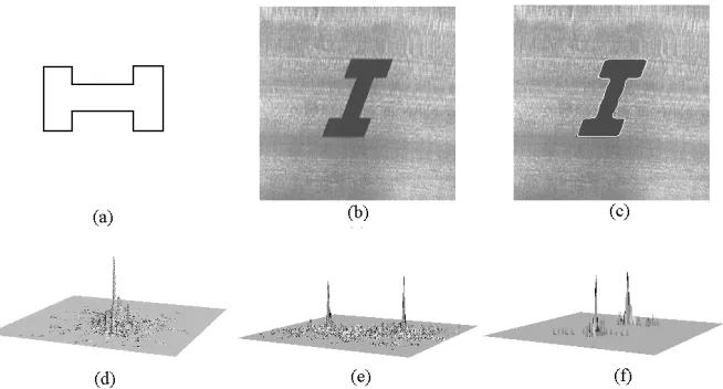
extraction process. The accumulators in Figures 1(d), 1(e) and 1(f) were obtained by gathering evidence according to equation (9). These accumulators have well-defined peaks which define an accurate value of the parameters of the transformation. The pair of peaks in the accumulators of Figures 1(d) and 1(e) show that the matching allows two solutions that correspond to mirror transformations. The shape defined by these transformations is shown in Figure 1(f) superimposed on the original image.

Figure 1. Example of the extraction process. (a) Model shape. (b) Raw image.

(c) Extraction result. (d)Evidence of the translation parameters. (e) Evidence of two transformation parameters. (f) Evidence of two transformation parameters.

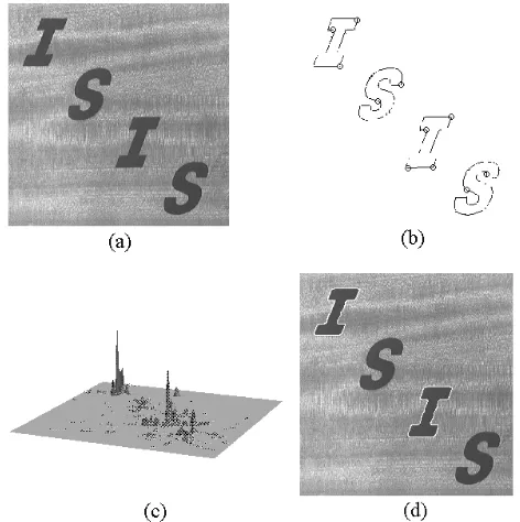
Figure 2. Example of wrong extraction for two primitives. (a) Raw image. (b) Edge

The well-defined peaks in the accumulators of the example in Figure 1 show that the mapping in equation (9) provides an effective approach for gathering evidence of arbitrary shapes under rigid transformations. However, the generality of the transformation can lead to incorrect results. This case is illustrated in the example shown in Figure 2. This example was obtained by considering the same gathering process as the one used in the example in Figure 1. The only difference is that the input image contains an extra object. However, the accumulator for the location parameters in Figure 2(d), contains two well-defined peaks which suggest that both objects correspond to the model. Furthermore, the largest peak is associated with the letter "S", not the letter "I", so the wrong shape/transformation is actually selected. An analysis of the evidence gathering process shows that the incorrect location is due to the wrong values produced by the lack of discriminatory power of the invariance constraints.

In order to obtain a good result it is necessary to include the constraint in equation (11). The effectiveness of this constraint is illustrated in the example in Figure 3. The image in Figure 3(a) contains four objects, two of which are instances of the model shape. Figure 3(b) shows the edges used in the gathering evidence process. Figure 3(c) shows the accumulator obtained by constraining the gathering process. The accumulator presents two well-defined peaks that provide an accurate estimate of the position of the instances of the primitive. Figure 3(d) shows the result of the complete extraction process superimposed on the original image.

Figure 3. Example of the extraction process. (a) Raw image. (b) Edge points.

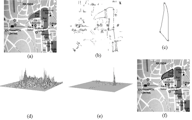
Figure 4. Example of the extraction process. (a) Raw image. (b) Edges. (c) Model shape. (d) Translation parameters accumulator. (e) Improved accumulator. (f)

Extraction result.

Figure 4 shows another example of the improvement achieved in the gathering process when the constraint in equation (11) is used. The edges in Figure 4(b) were obtained from the image in Figure 4(a) and used to gather evidence of the model shape in Figure 4(c). This model was actually defined by a continuous curve with 15 Fourier coefficients. Figure 4(d) shows the accumulator obtained according to equation (9). The accumulator in Figure 4(e) was obtained by including the constraint in equation (11). Comparison of the accumulator arrays accumulator in Figures 4(d) and (e) shows that prominent wrong peaks are completely eliminated, producing a single well-defined peak. Figure 4(f) shows the result (superimposed on black) obtained by the extraction technique.

6

Conclusions

The analytic formulation of the HT can be extended to extract arbitrary shapes under general transformations. The generality of this extension increases significantly the amount of false evidence. Geometric invariant features can be included in the formulation as an effective way of reducing the dimensionality of the transformation and to reduce the amount of false evidence gathered. However, the generality of the transformation can still produce an excessive amount of false evidence, potentially leading to incorrect results.

References

[1] J. Sklansky, On the Hough technique for curve detection, IEEE-T Computers 27:923-926 (1978).

[2] J. Illingworth, J. Kittler, A survey of the Hough transform, CVGIP 48:87-116 (1988).

[3] A.S. Aguado, M.E. Montiel, M.S. Nixon, Extracting arbitrary geometric primitives represented by Fourier descriptors, Proc. ICPR’96, pp. 547-551 (1996). [4] D.H. Ballard, Generalizing the Hough transform to detect arbitrary shapes, Patt.

Recog. 13:111-122 (1981).

[5] R.K.K. Yip, R.K.S Tam, D.N.K. Leung, Modification of the Hough transform for object recognition using a 2-dimensional array, Patt. Recog. 28(11):1733-1744 (1995).

[6] R-.C. Lo, W.-H. Tsai, Perspective-transformation-invariant generalized Hough transform for perspective planar shape detection and matching, Patt. Recog. 30(3):383-396 (1997).

[7] S.Y. Yuen, C.H. Ma, An investigation of the nature of parameterization for the Hough transform, Patt. Recog. 30(6):1009-1040 (1997).

[8] W.E.L. Grimson, D.P. Huttenlocher, On the sensitivity of the Hough transform for object recognition, IEEE-T PAMI 12(3):255-274 (1990).

[9] W.E.L. Grimson, D.P. Huttenlocher, On the verification of the hypothesized matches in model-based recognition, IEEE-T PAMI 13:1201-1213 (1991).

[10]S.M. Bhandarkar, M. Su, Sensitiviy analysis for matching and pose computation using dihedral junctions, Patt. Recog. 24:505-513 (1991).

[11]C.S. Chakravarthy, R. Kasturi, Pose clustering on constraints for object recognition, CVPR'91, pp. 16-21 (1991).

[12]Y. Lamdan, H.J. Wolfson, On the error analysis of 'Geometric Hashing', CVPR'91, pp. 22-27 (1991).

[13]A.S. Aguado, M.E. Montiel, M.S. Nixon, Bias error analysis of the generalised Hough transform, Journal of Mathematical Imaging and Vision 12(1):25-42 (2000).

[14]A. Califano, R. Mohan, Multidimensional indexing for recognizing visual shapes, IEEE-T PAMI 16(4):373-392 (1994).

[15]S. Tsuji, F. Matsumoto, Detection of ellipses by a modified Hough transform, IEEE-T Computers 27:777-781 (1978).

[16]J.H. Yoo, I.K. Sethi, An ellipse detection method from the polar and pole definition of conics, Patt. Recog. 26(2):307 -315 (1993).

[17]W.-Y. Wu, M.-J.J. Wang, Elliptical object detection by using its geometric properties, Patt. Recog. 26(10):1499-1509 (1993).