Online Full Text

Abstract— Accurately predicting cancer patient survival

rates is crucial for cancer prognosis. TNM is a widely used 3-predictor based prediction model that involves Tumor extent, lymph Node involvement and Metastasis. However, using only three prognostic factors limits its prediction accuracy. To overcome this limitation, machine learning techniques and statistical analysis have been deployed. For example, the Ensemble Algorithm of Clustering of Cancer Data (EACCD) has been developed by Chen et al. with the improved survival rate prediction. EACCD first uses Partitioning Around Medoids (PAM) clustering algorithm to calculate dissimilarity for survival curves and then refine it with an ensemble average to obtain so-called learnt dissimilarity. In this paper, we propose a Group Algorithm for Cancer Data (GACD) by redefining the learnt dissimilarity with weights to improve algorithm efficiency. In addition, we investigate how GACD depends on the clustering algorithms with the Fuzzy clustering algorithm and devise a geometrical metric to evaluate the quality of the grouping results. Furthermore, we evaluate the consistency of grouping results from two nearly equal-sized datasets. Our experimental results show that the Fuzzy and PAM algorithms produce different grouping results, weighted dissimilarity method improves the overall accuracy, and the grouping results from two nearly equal-size datasets have almost consistent survival curves and dendrograms.

Index Terms—Survival Rate, Prediction, TNM, Clustering

Algorithm

I. INTRODUCTION

he American Joint Committee on Cancer (AJCC) classification proposed that the same anatomic and histology share similar growth and outcomes [1]. Many analysis methods of cancer patient data adhere to this assumption and therefore a classification scheme becomes crucial for cancer diagnosis. A staging-based classification scheme, TNM system involves three important prognostic factors, local tumor growth (T), lymph nodes (N) and metastasis (M) [1]. However, as in-depth studies and significant progresses were made in the current cancer research, three prognostic factors (T, N, and M) are not enough for accurately predicting the survival outcome. For better prognosis and treatment, several approaches intend to expand the TNM system by involving more prognostic factors [2]-[6].

An improved prognostic system usually consists of groups of patients, and the patients in the same group have similar survival outcomes. Hence, designing efficient clustering algorithms to group similar patients is quite useful for the survival prediction. Since cancer data include a large amount of censored observations, applying traditional clustering

Manuscript received December 28, 2012; revised January 28, 2014. R. Qi and S. Zhou are with the Department of Electrical and Computer Science, University of Maryland, Baltimore County, Baltimore, MD, 21250, USA, e-mail: [email protected], [email protected]

algorithm on the censored data leads to distorted grouping result [7]. Hence, there is a need to develop a clustering algorithm cooperated with censored data. Based on the assumption that patients with the same levels of prognostic factors have similar survival outcomes, finding groups in patients is therefore equivalent to finding groups in all the available combinations of levels of prognostic factors [2]. For the survival times of the patients in one combination, an overview of the survival distribution in their life history can be portrayed as a survival curve by the Kaplan-Meier Estimator [8]. The dissimilarity between two survival curves is usually estimated by the log-rank test [9]. Both techniques, Kaplan-Meier Estimator and log-rank test, take censored data into account. Consequently, the aim for a prognostic system to predict the survival outcome reduces to group survival curves.

The ensemble algorithm of clustering of cancer data (EACCD) was developed to improve the TNM systems [2]. The patients are first grouped by the combinations of levels of prognostic factors, which significantly reduce the size of the dataset. The extracted combinations are then grouped by a hierarchical clustering algorithm. The selection of clustering criterions in the hierarchical clustering has been discussed in [7], which indicates that complete or average linkage yields a reasonable grouping result while single linkage could generate misleading ones. The measure of dissimilarity is another essential factor that impacts the grouping result. The initial dissimilarity of combinations is measured by the log-rank test. Other tests such as Gehan-Wilcoxon’s test, Tarone and Ware’s test generate similar results to the rank test [7]. As the test statistic of the log-rank test is sensitive to the size of the combination [7], the initial dissimilarity is standardized by an ensemble clustering method referred to as the learning step. The EACCD algorithm [2] intended to calculate the ensemble average based on a large number of random clustering outputs through voting. However, if an un-randomized PAM algorithm is employed, we can obtain the reasonable accuracy with the number of runs less than the number of combinations. Considering the limited number of votes during the learning step, we should find a way to improve the accuracy of dissimilarity measurement. We consider the fact that the probability of a combination falling into a cluster depends on the number of available clusters. It is evident that the probability of two combinations falling into the same cluster is higher in the 2-cluster configuration than in the 11-cluster configuration. Therefore, these two clustering configurations should not be treated equally. To address this issue, we redefine the measurement of the learnt dissimilarity by taking each configuration only once and adding the weight to include the dependency of grouping probability mentioned above so as to improve the quality of the measurement.

A Comparative Study of Algorithms for

Grouping Cancer Data

Ran Qi, Shujia Zhou

Within the learning step, different clustering algorithms can be employed for calculating dissimilarity. There are two restrictions on selecting clustering algorithms: (1) it needs to be a partitioning algorithm; (2) it can operate on the dissimilarity matrix. Since the hierarchical clustering is not appropriate for a single partitioning of the dataset, and the dissimilarity is not measured by the Euclidean distance, hierarchical clustering or K-Means clustering algorithm is not applicable. Fuzzy clustering algorithm [10] satisfies both restrictions.

The experimental results of the EACCD for various types of cancer [2] [7] [11] and an analysis of the impacts of different algorithm settings [7] have been previously reported. In addition, it is known that the outcome of clustering algorithms depends on the object functions and is also affected by the local minimum issues. So far, there exists no quantitative metric to evaluate the quality of these results. We devise a geometrical metric based on the enclosed area between survival curves and show that it can effectively compare the quality of various grouping results.

The rest of the paper is organized as follows. In section 2, we review some related concepts in survival analysis and clustering algorithms. In section 3, we define a weighted learning dissimilarity in the learning step. A newly devised evaluation metric for grouping results is proposed in section 4. In section 5, we present dataset as well as the algorithms used in the experiments. We describe and analyze experimental results in section 6 and conclude in section 7.

II. BACKGROUND

The two essential elements in the EACCD are survival analysis and clustering procedures. In this section, we first provide a brief introduction on survival analysis and then describe clustering algorithms.

A. Survival analysis

Survival analysis includes numerous statistical methods for analyzing survival times [12][13]. The survival time is an important element in the survival analysis that measures the length of the time period from the diagnosis of a disease to a specific event (e.g., death, lost to follow-up). The cancer data usually include censored and uncensored times. The censored time is not equal to the exact survival time. In survival analysis, both censored and uncensored times have to be taken into account.

There are two commonly used techniques in survival analysis: Kaplan-Meier estimator and log-rank test. The Kaplan-Meier estimator provides an overview of survival distribution with estimated survival probabilities. The log-rank test typically evaluates whether the survival distributions for two groups of patients are statistically different. Both methods can operate on the censored and uncensored times. B. Clustering algorithms

Clustering techniques are used to find groups or clusters from a large amount of data objects so that the objects in the same cluster are as similar as possible. Clustering has been applied to various fields including medicine. Commonly used clustering procedures include partitioning approaches and hierarchical approaches. The partitioning algorithm divides a given dataset into a series of subsets based on a certain

criterion while the hierarchical method organizes the dataset into a representation that reveals the intrinsic hierarchical structure of the dataset.

PAM algorithm is a typical partitioning clustering algorithm. It tries to find the centrally located object called medoid in each cluster. The remaining objects are then assigned to the closest medoid. The goal of the algorithm is to minimize the average dissimilarity of objects to their closest medoids. The standard PAM algorithm includes BUILD phase and SWAP phase [10]. The BUILD phase determines initial medoids, and the SWAP phase intends to improve the quality of clustering result by swapping medoids with non-medoids. Both the BUILD and SWAP phases produce deterministic results. PAM is a hard partitioning clustering algorithm, which can operate on a dissimilarity matrix dataset. It satisfies the two restrictions on the candidate algorithms for the EACCD and is the original algorithm used in the EACCD.

Fuzzy algorithm is a partitioning clustering method that allows some ambiguity in the data instead of a crispy partition. Each object can be assigned to multiple clusters by the degree of belongings. A fuzzy clustering becomes a hard clustering when each object is assigned to the cluster where its degree of belongings is the maximum. Fuzzy algorithm can either operate on the dissimilarity matrix dataset or dimensional data matrix. Therefore, Fuzzy can be treated as an alternative algorithm of the PAM [14] in the EACCD. The Fuzzy function implemented in R [15][16] limits the number of clusters from 1 to n/2-1 where n is the number of objects. The detailed algorithm can be found in Kaufman’s book [10].

Hierarchical clustering seeks to build a set of nested clusters that are organized as a tree. It can be either bottom up approach that starts from each individual object and merges the closest clusters in each step, or top down approach where splitting is recursively performed. The output of hierarchical clustering is usually presented in a dendrogram. EACCD can use any linkage function to build up the tree in a bottom up manner. The previous study of linkage functions shows that the complete and average are the preferred linkages [7].

III. ENSEMBLE ALGORITHM WITH WEIGHTED LEARNING DISSIMILARITY

EACCD computes the learnt dissimilarity based on multiple runs of different clustering algorithms. When only one clustering algorithm (e.g., PAM) is used, variable output is required from the EACCD algorithm. However, a clustering algorithm without variable output can still be used with EACCD. In this section, we propose a weighted learning dissimilarity computed by using the standard PAM algorithm that generates deterministic results. Our approach only requires n-2 runs of the PAM where n is the number of combinations, thus significantly reducing the computational time.

A. EACCD Algorithm

initial dissimilarities by the log-rank test; (c) learn new dissimilarities by a sequence of PAM procedures; (d) use hierarchical clustering with average linkage to produce groups of patients. In EACCD, the survival curves of combinations are plotted by the Kaplan-Meier estimator. B. Grouping Algorithm for Cancer Data

The dissimilarity between combinations is measured by the log-rank test and multiple partitioning procedures. Different implementations of the partitioning algorithm could have different impacts on the measure of dissimilarity. The EACCD algorithm requires a large number of random clustering outputs to calculate an ensemble average as the learnt dissimilarity. In our approach, the standard PAM can be used to generate n-2 partitioning outputs, and the new learnt dissimilarity is defined as the average value of the weighted partitioning outputs.

The calculation for dissimilarity is done in the steps (b) and (c) of the original EACCD. Step (b) initializes the dissimilarity by the log-rank test statistic, and step (c) standardizes it to the learnt dissimilarity. The detailed learning step is as follows: n combinations {x1, x2, … , xn} are divided into k clusters by the PAM algorithm, and k is randomly selected from 2 to n-1. This procedure is repeated for m times (m is a large number such as 10000) in which each iteration produces a partition of these combinations. Thus m partitions are obtained from m runs of PAM. For the lth run, the dissimilarity of combinations is defined as dl(i,j) =1 if the lth partition assigns xi and xj into different cluster and dl(i,j) = 0 otherwise. The learnt dissimilarity is based on the results of all m runs:

𝑑𝑖𝑠(𝑥𝑖, 𝑥𝑗) =

∑𝑚𝑙=1𝑑𝑙(𝑖,𝑗)

𝑚 (1)

The learnt dissimilarity is the probability of two combinations assigned to different clusters. If two combinations are assigned to the same cluster for the majority of iterations, the learnt dissimilarity will approach to 0. It is therefore very likely that the patients from these two combinations share one survival curve. Note that (1) is designed for any implementation (of the PAM algorithm) that provides a “random” output.

When an un-randomized PAM algorithm (e.g., the standard PAM) is utilized, equation (1) can be greatly simplified. Let n denotes the total number of combinations. A partition with k clusters corresponds to one possible partitioning output. If k can be selected from 2 to n-1, the standard PAM algorithm can only provide up to n-2 different partitioning outputs. Therefore, we can modify the learnt dissimilarity (1) into (2):

𝑑𝑖𝑠2(𝑥𝑖, 𝑥𝑗) =∑ 𝑑𝑘(𝑖,𝑗)

𝑛−1 𝑘=2

𝑛−2 (2)

It is evident that intensity of dissimilarity is not the same over all the clustering configurations. For example, the probability of two combinations falling into the same cluster is higher in the 2-cluster configuration than in the 11-cluster configuration. However, equation (2) treats all the configurations equally. To consider the difference in the intensities of dissimilarity among these clustering configurations, we add weights to the dissimilarity as shown in (3)

𝑑𝑖𝑠3(𝑥𝑖, 𝑥𝑗) = ∑𝑛−1𝑘=2𝑤𝑘𝑑𝑘(𝑖, 𝑗) (3)

In (3), wk is the weight such as 0≤wk≤1 and ∑𝑛−1𝑘=2𝑤𝑘 = 1.

The weight quantifies the likelihood that two combinations fall into the different clusters. We show how to calculate the weights below.

It is obvious that the larger the number of clusters is, the more likely two objects will be assigned to different clusters. It implies that the intensity of the learnt dissimilarity is low. Hence, a smaller weight should be assigned to 𝑑𝑘(𝑖, 𝑗) with a

larger k. Assuming the weight is inversely proportional to k, and then we have:

𝑤𝑘 = 𝐶 ∗1_𝑘 (4)

where C is a constant. From (4) and ∑𝑛−1_𝑘=2(𝑤_𝑘)= 1, C is determined by

𝐶 = _∑𝑛−11_{(1 𝑘⁄ )}

𝑘=2 (5)

Using (3), (4) and (5), we see that dis3 can be written as:

𝑑𝑖𝑠3(𝑥𝑖, 𝑥𝑗) = ∑ _𝑘∗∑𝑛−11_{(1 𝑖)⁄} 𝑖=2 𝑑𝑘(𝑖, 𝑗)

𝑛−1

𝑘=2 (6)

IV. EVALUATION METRIC

The EACCD algorithm has been applied to studies for lung cancer [2], breast cancer [7] and melanoma [11]. However, there is no quantitative metric to evaluate the quality of grouping results. Currently, the commonly used evaluation is simply done by visually comparing survival curves. The closest curves are expected to be combined first. However, this method is error-prone and subjective especially when the curves are close.

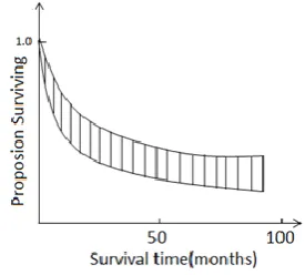
We propose a geometrical metric to evaluate grouping results of GACD by quantifying the dissimilarity between two curves with the area enclosed between these two curves as illustrated in Fig. 1. The dissimilarity of two curves is measured as the shaded area as shown in Fig. 1.

Fig. 1. Geometrical dissimilarity metric

V. EXPERIMENTS

In this section, we performed a series of experiments to assess the impact of different clustering algorithms on the grouping results. In addition, we will verify the effectiveness of our weighted dissimilarity and geometrical metric, and consistency of grouping results.

A. Dataset

The dataset used in this study is the SEER data [16] that contains 202,219 records of breast cancer patients from the year 1990 to 2000. The factors we studied include tumor size (T) and node status (N). For convenience, the combination is represented by the levels of the factors, as shown in Table 1. For example, 32 denotes the patients for whom tumor size is greater than 5cm and 1~3 nodes contain tumor. There are 12 combinations in our dataset after discarding the combinations consisting of less than 100 patients.

TABLE I

DEFINITION OF T AND N IN BREAST CANCER DATASET

Factors Category Level

Tumor size (T)

T ≤ 2cm 1

2cm < T ≤ 5 cm 2

T > 5cm 3

Node status (N)

No positive nodes 1

1~ 3 nodes 2

4 ~ 10 nodes 3

> 10 nodes 4

To evaluate the consistency of the GACD grouping results from the same type of cancer data, we split the whole dataset into two nearly equal-sized subsets. The data in the two subsets, Datset1 and Dataset2, are randomly selected from the original dataset. The consistency of survival curves and dendrograms from these two subsets are used to evaluate the performance of the GACD algorithm.

B. Setting of the algorithms

The PAM and Fuzzy algorithms will be used in our experiments. The initial dissimilarity is generated by the log-rank test. In the learning step, we use the Fuzzy function implemented in R, therefore the number of clusters by the Fuzzy algorithm is limited from 1 to n/2-1. Equation (2) can be modified to

𝑑𝑖𝑠4(𝑥𝑖, 𝑥𝑗) =

∑𝑛/2−1_𝑘=2 𝑑_𝑘(𝑖,𝑗)

𝑛/2−2 (7)

and modify the (6) to

𝑑𝑖𝑠5(𝑥𝑖, 𝑥𝑗) = ∑ _𝑘∗∑𝑛/2−11 _{(1 𝑖)⁄} 𝑖=2

𝑑𝑘(𝑖, 𝑗) 𝑛/2−1

𝑘=2 (8)

The dissimilarity functions used in our study are as follows:

1) Using the Fuzzy algorithm and (7) and (8) 2) Using the PAM algorithm and (7) and (8)

3) Combining the results from both the Fuzzy and PAM algorithms, using (7) and (8)

4) Using the PAM algorithm and (2) and (6)

Eight experiments have been carried out based on the dissimilarity functions above. There are four experiments

with weighted strategy ((6) and (8)) and four experiments without the weight ((2) and (7)). In addition, we perform one more experiment that omits the learning step to compare it with the eight experiments above.

VI. RESULTS AND ANALYSIS

A. Compare results from different clustering algorithms The experimental results indicate that the structures of the dendrograms are similar to each other regardless of whether weight is applied. The merging order is the same, while the sequence of fusion levels in the dendrogram are slightly different. So we only presented the dendrograms generated by the weighted learnt dissimilarity.

(a) Using Fuzzy algorithm and (8)

(b) Using PAM algorithm and (8)

(c) Using Fuzzy+PAM algorithm and (8)

(d) Using PAM algorithm and (6)

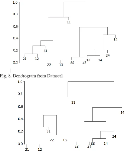
In the dendrogram shown in Fig. 2 (a), the Fuzzy algorithm is employed for computing the learnt dissimilarity, and (8) is used as the dissimilarity measure between xi and xj. Starting from the bottom level, the dissimilarity in each of following groups is 0.0: (21, 31, 12), (32, 23), (33, 24, 34), and (22, 13). Since the combinations with the lowest dissimilarity are merged as a group, we have four groups of patients at the dissimilarity 0.0. The next two merges occur at 0.16 between (21, 31, 12) and 11, and between (33, 24, 34) and 14. Moving upwards along the fusion level, all combinations are finally merged together at the highest level of dissimilarity. In order to make a fair comparison of the Fuzzy and PAM algorithms, the dendrogram computed by PAM and (8) is shown in Fig. 2(b). Fig. 2(c) shows the dendrogram corresponding to the case where the learnt dissimilarity is the average of the learnt dissimilarities calculated with the Fuzzy and PAM algorithms. Although (6) cannot be applied to the Fuzzy algorithm, it can be used for the PAM algorithm that can deal with the number of clusters from 2 to n-2. The dendrogram in Fig. 2(d) is the grouping result for this case.

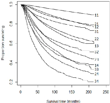
Fig. 3. Kaplan-Meier survival curves for 12 combinations

Next we compare the quality of dendrograms. Each dendrogram exhibits a relationship among the survival curves. The affinity between a dendrogram and the associated survival curves is an important factor for the quality evaluation. If the merging pattern in the dendrogram is similar to the merging order of the associated curves, this dendrogram has a good representation. To evaluate the merging pattern of a dendrogram, we only need to examine each dissimilarity level where a fusion occurs in a bottom-up manner. As an example, Fig. 2 (d) illustrates that (32, 23) is the first group merged at the lowest dissimilarity level 0.0. Therefore (32, 23) constitutes the first group of patients. The next merge is between group (21, 12) and (33, 14), since they have the second smallest dissimilarity. It is evident from the dendrogram that the order of merging reflects the geometric affinity between the curves. In other words, if two curves are closer to each other, their associated combinations will be merged earlier in the dendrogram. As seen in Fig. 3, the curve closest to that of combination 21 is 12 while (21, 12) is the first group merged at the bottom level in the dendrogram. The next closest curve to the group (21, 12) is 31 while 31 is merged with (21, 12) in the next upper level. Through examining the dendrogram, it is clear that the geometric

affinity among survival curves is able to reflect the merging order in the dendrogram from the bottom to the top level.

TABLE II

COMPARISON OF CORRELATION COEFFICIENTS

Algorithms Correlation coefficients Without weight With weight

Fuzzy 0.9328 (7) 0.9365 (8)

PAM 0.8356 (7) 0.8771 (8)

Fuzzy + PAM 0.8141 (7) 0.8334 (8)

PAM 0.8210 (2) 0.8922 (6)

Omit learning step 0.7066

However, assessing the dissimilarity between two survival curves through eyes is subjective and error-prone. Therefore, solely relying on observation cannot adequately examine the quality of grouping results represented with the dendrograms in Fig. 2. Our newly proposed geometrical metric appears to be able to effectively address this problem. With the merging order, we can obtain a sequence of increasing dissimilarity levels along with the geometrical dissimilarities from the associated survival curves as shown in Fig. 3. Table 2 lists the linear correlation coefficients for each case. A larger correlation coefficient implies a better grouping quality in terms of the dissimilarity of survival curves.

Fig. 4. Evaluation of the grouping results

Fig. 4 reveals that different clustering algorithms yield different grouping results. In terms of correlation, it appears that the Fuzzy algorithm provides a better result compared with the PAM. One possible reason for different grouping results is that the solutions from both PAM and Fuzzy algorithms correspond to local minimums.

Table 2 indicates that adding weights in the learning step leads to a higher correlation in all the cases, even though their dendrograms have similar structures. It is expected that the effect of adding weights becomes more significant as the number of combinations increases.

Fig. 5. Evaluation of the grouping result without learning step

B. Compare results from two nearly equal-sized datasets

We compare and analyze survival curves and dendrograms obtained from two datasets. Each dataset includes 12 combinations (same as the original dataset). Their survival curves are shown in Fig. 6 and Fig.7. Comparing surviving curves in Fig. 6 and Fig. 7, we observe that except the combinations 13 and 22, the order of survival curves is almost identical. Their corresponding dendrograms are shown in Fig.8 and Fig. 9. As shown in Table III and IV, there are some differences in the merging orders between the two data sets. For example, the group of (33, 14, 24) in Dataset1 first merges to 34 and then (32, 23). But (33, 14, 24) in Dataset2 first merges (32, 23) and then 34. After 12 curves reduce to 4 curves, the grouping results are identical.

Fig. 6. Kaplan-Meier survival curves from Dataset1

Fig. 7. Kaplan-Meier survival curves from Dataset2

Fig. 8. Dendrogram from Dataset1

Fig. 9. Dendrogram from Dataset2

TABLE III

MERGING ORDER FROM DATASET1 1 [0][1][2][3][4][5][6][7][8][9][10][11] 2 [0][1][2][3,8][4][5][6][7][9][10][11] 3 [0][1,4][2][3,8][5][6][7][9][10][11] 4 [0][1,4][2][3,8][5,9][6][7][10][11] 5 [0,11][1,4][2][3,8][5,9][6][7][10] 6 [0,11][1,4][2][3,8][5,9,6][7][10] 7 [0,11,2][1,4][3,8][5,9,6][7][10] 8 [0,11,2,3,8][1,4][5,9,6][7][10] 9 [0,11,2,3,8][1,4][5,9,6,7][10] 10 [0,11,2,3,8][1,4,5,9,6,7][10] 11 [0,11,2,3,8,10][1,4,5,9,6,7] 12 [0,11,2,3,8,10,1,4,5,9,6,7]

TABLE IV

MERGING ORDER FROM DATASET2 1 [0] [1] [2] [3] [4] [5] [6] [7] [8] [9] [10] [11] 2 [0,11] [1] [2] [3] [4] [5] [6] [7] [8] [9] [10] 3 [0,11] [1,4] [2] [3] [5] [6] [7] [8] [9] [10] 4 [0,11] [1,4] [2] [3] [5,9] [6] [7] [8] [10] 5 [0,11] [1,4] [2] [3,8] [5,9] [6] [7] [10] 6 [0,11] [1,4] [2] [3,8] [5,9,6] [7] [10] 7 [0,11,2] [1,4] [3,8] [5,9,6] [7] [10] 8 [0,11,2] [1,4,5,9,6] [3,8] [7] [10] 9 [0,11,2,3,8] [1,4,5,9,6] [7] [10] 10 [0,11,2,3,8] [1,4,5,9,6,7] [10] 11 [0,11,2,3,8,10] [1,4,5,9,6,7] 12 [0,11,2,3,8,10,1,4,5,9,6,7]

whole dataset, and listed in Tables VI, VII and VIII, respectively. Comparing the P values in Table V against those in Tables VI, VII and VIII, it is found that the P values in Table V are much larger than those in Table VI, VII and VIII. That is, the differences between the survival curves in Dataset1 and Dataset2 are small since a smaller value of a log-rank test statistic or a larger value of P value shows a stronger evidence of no difference.

Based on the results of comparing merging order and P values discussed above, we believe that GACD is capable of generating consistent grouping results.

TABLE V

THE DIFFERENCE IN SURVIVAL CURVES FROM TWO DATASETS Log-rank test P value

[0] 2.1 0.15

[1] 0 0.962

[2] 0.2 0.636

[3] 0.8 0.379

[4] 0.1 0.78

[5] 0.1 0.814

[6] 1 0.316

[7] 0.1 0.718

[8] 1.4 0.233

[9] 0 0.983

[10] 0.1 0.804

[11] 0.1 0.748

TABLE VI

P VALUES OF ALL PAIRS OF 12 COMBINATIONS FROM DATASET1 [0] [1] [2] [3] [4] [5] [6] [7] [8] [9] [10] [11] [0] 0.00 0.00 0.00 0.00 0.00 0.00 0.00 0.00 0.00 0.00 0.00 0.00 [1] 0.00 0.00 0.00 0.00 0.19 0.00 0.00 0.00 0.00 0.00 0.00 0.00 [2] 0.00 0.00 0.00 0.00 0.00 0.00 0.00 0.00 0.00 0.00 0.00 0.00 [3] 0.00 0.00 0.00 0.00 0.00 0.00 0.00 0.00 0.00 0.00 0.01 0.00 [4] 0.00 0.19 0.00 0.00 0.00 0.00 0.00 0.00 0.00 0.00 0.00 0.00 [5] 0.00 0.00 0.00 0.00 0.00 0.00 0.00 0.00 0.00 0.00 0.00 0.00 [6] 0.00 0.00 0.00 0.00 0.00 0.00 0.00 0.00 0.00 0.55 0.00 0.00 [7] 0.00 0.00 0.00 0.00 0.00 0.00 0.00 0.00 0.00 0.00 0.14 0.00 [8] 0.00 0.00 0.00 0.00 0.00 0.00 0.00 0.00 0.00 0.00 0.00 0.00 [9] 0.00 0.00 0.00 0.00 0.00 0.00 0.55 0.00 0.00 0.00 0.00 0.00 [10] 0.00 0.00 0.00 0.01 0.00 0.00 0.00 0.14 0.00 0.00 0.00 0.00 [11] 0.00 0.00 0.00 0.00 0.00 0.00 0.00 0.00 0.00 0.00 0.00 0.00

TABLE VII

P VALUES OF ALL PAIRS OF COMBINATIONS FROM DATASET2 [0] [1] [2] [3] [4] [5] [6] [7] [8] [9] [10] [11] [0] 0.00 0.00 0.00 0.00 0.00 0.00 0.00 0.00 0.00 0.00 0.00 0.00 [1] 0.00 0.00 0.00 0.00 0.19 0.00 0.00 0.00 0.00 0.00 0.00 0.00 [2] 0.00 0.00 0.00 0.00 0.00 0.00 0.00 0.00 0.00 0.00 0.00 0.00 [3] 0.00 0.00 0.00 0.00 0.00 0.00 0.00 0.00 0.00 0.00 0.01 0.00 [4] 0.00 0.19 0.00 0.00 0.00 0.00 0.00 0.00 0.00 0.00 0.00 0.00 [5] 0.00 0.00 0.00 0.00 0.00 0.00 0.00 0.00 0.00 0.00 0.00 0.00 [6] 0.00 0.00 0.00 0.00 0.00 0.00 0.00 0.00 0.00 0.55 0.00 0.00 [7] 0.00 0.00 0.00 0.00 0.00 0.00 0.00 0.00 0.00 0.00 0.14 0.00 [8] 0.00 0.00 0.00 0.00 0.00 0.00 0.00 0.00 0.00 0.00 0.00 0.00 [9] 0.00 0.00 0.00 0.00 0.00 0.00 0.55 0.00 0.00 0.00 0.00 0.00 [10] 0.00 0.00 0.00 0.01 0.00 0.00 0.00 0.14 0.00 0.00 0.00 0.00 [11] 0.00 0.00 0.00 0.00 0.00 0.00 0.00 0.00 0.00 0.00 0.00 0.00

TABLE VIII

P VALUES OF ALL PAIRS OF COMBINATIONS FROM THE WHOLE DATASET [0] [1] [2] [3] [4] [5] [6] [7] [8] [9] [10] [11] [0] 0.00 0.00 0.00 0.00 0.00 0.00 0.00 0.00 0.00 0.00 0.00 0.00 [1] 0.00 0.00 0.00 0.00 0.01 0.00 0.00 0.00 0.00 0.00 0.00 0.00 [2] 0.00 0.00 0.00 0.00 0.00 0.00 0.00 0.00 0.00 0.00 0.00 0.00 [3] 0.00 0.00 0.00 0.00 0.00 0.00 0.00 0.00 0.00 0.00 0.00 0.00 [4] 0.00 0.01 0.00 0.00 0.00 0.00 0.00 0.00 0.00 0.00 0.00 0.00 [5] 0.00 0.00 0.00 0.00 0.00 0.00 0.00 0.00 0.00 0.00 0.00 0.00 [6] 0.00 0.00 0.00 0.00 0.00 0.00 0.00 0.00 0.00 0.30 0.00 0.00 [7] 0.00 0.00 0.00 0.00 0.00 0.00 0.00 0.00 0.00 0.00 0.01 0.00 [8] 0.00 0.00 0.00 0.00 0.00 0.00 0.00 0.00 0.00 0.00 0.00 0.00 [9] 0.00 0.00 0.00 0.00 0.00 0.00 0.30 0.00 0.00 0.00 0.00 0.00 [10] 0.00 0.00 0.00 0.00 0.00 0.00 0.00 0.01 0.00 0.00 0.00 0.00 [11] 0.00 0.00 0.00 0.00 0.00 0.00 0.00 0.00 0.00 0.00 0.00 0.00

VII. CONCLUSION

To improve efficiency and accuracy in predicting cancer patient survival rates, we introduce a Grouping Algorithm for Cancer Data (GACD). Experiments show that the grouping results of GACD depend on clustering algorithms. In addition, adding weights in the learnt dissimilarity calculation improves the quality of the grouping result. Moreover, a geometrical metric defined as the area enclosed by two survival curves is effective in assessing the quality of the grouping results. Finally, the grouping results generated by GACD show a good consistency between the two nearly equal-sized datasets.

ACKNOWLEDGMENT

The authors wish to thank Dr. Dechang Chen for helpful discussion.

REFERENCES

[1] F. L. Greene, C. C. Compton, A. G. Fritz, J. P. Shah, and D. P.Winchester, Eds., AJCC Cancer Staging Atlas, Springer, New York, NY, USA, 2006

[2] D. Chen, K. Xing, D. Henson, L. Sheng, A.M. Schwartz, and X. Cheng, “Developing Prognostic Systems of Cancer Patients by Ensemble Clustering”. Journal of Biomedicine and Biotechnology, vol. 7, 2009

[3] K. Xing, D. Chen, D. Henson, and L. Sheng, “A clustering-based approach to predict outcome in cancer patients,” the 6th International Conference on Machine Learning and Applications (ICMLA ’07), pp. 541–546, Cincinnati, Ohio, USA, December 2007.

[4] H.B. Burke, D.E. Henson, “Criteria for prognostic factors and for an enhanced prognostic system”. Cancer. vol. 72, 1993, pp. 3131-3135

[5] H.B. Burke, P.H. Goodman, D.B. Rosen, D.E. Henson, J.N. Weinstein, F.E. Harrell, J.R. Marks, D.P. Winchester, D.G. Bostwick, “Artificial neural networks improve the accuracy of cancer survival prediction” Cancer, vol 79, 1997, pp. 857-862 [6] H.B. Burke, “Outcome prediction and the future of the TNM

staging system”, Journal of the National Cancer Institute, vol 96, 2004, pp. 1408-1409

[7] D. Wu, L. Sheng, E. Xu, K. Xing, D. Chen, “Analysis of an Ensemble Algorithm for Clustering Cancer Data”, IEEE International Conference on Bioinformatics and Biomedicine Workshops (BIBMW), 2012, pp. 754-755

[8] E.L. Kaplan, P. Meier, “Nonparametric estimation form incomplete observations”, Journal of the American Statistical Association, val. 53, no.282, 1958, pp. 457-481

[9] D.P. Harrington and T.R. Fleming, “A class of rank test procedure for censored survival data”, Biometrika, vol.69, 1982, pp. 553-566

[10]L. Kaufman, P.J. Rousseeuw, Finding groups in data, An introduction to cluster analysis Edegem, 1989, Belgium [11]D. Wu, C. Yang, S. Wong, J. Meyerle, B. Zhang, D. Chen, “An

Examination of TNM Staging of Melanoma by a Machine Learning Algorithm”. International Conference on Computerized Healthcare, 2012

[12]V. Bewick, L. Cheek, J. Ball (2004) “Survival analysis”, Available: http://www.ncbi.nlm.nih.gov/pmc/articles/PMC10

65034/

[13]D.G. Kleinbaum, M. Klein, Survival Analysis, a self-learning text, third edition, Springer, 2012, New York

[14]Data Mining Algorithms In R/Clustering/ Partitioning Around Medoids (PAM), Available: http://en.wikibooks.org/wiki/ Data_Mining_Algorithms_In_R/Clustering/Partitioning_Arou

[15]Fuzzy Analysis Clustering in R package, Available:

http://stat.ethz.ch/R-manual/R-patched/library/cluster/html/ fanny.html

[16]The R Project for Statistical Computing, Available:

http://www.r-project.org/

[17]A.D. Robert, The complete idiot’s guide to statistics, second edition, Alpha, New York, 2007, pp. 312-314