The Canadian Journal of Statistics Vol. 28, No. ?, 2000, Pages ???-??? La revue canadienne de statistique
Likelihood inference for small
variance components
Steven E. STERN and A. H. WELSH
Key words and phrases: boundary, likelihood-based inference, local asymptotics, maximum likelihood estimation, REML, variance components, Wald test.
AMS 1991 subject classifications: Primary 62F12; secondary 62F30.
ABSTRACT
The authors explore likelihood-based methods for making inferences about the compo-nents of variance in a general normal mixed linear model. In particular, they use local asymptotic approximations to construct confidence intervals for the components of vari-ance when the components are close to the boundary of the parameter space. In the process, they explore the question of how to profile the restricted likelihood (REML). Also, they show that general REML estimates are less likely to fall on the boundary of the parameter space than maximum likelihood estimates and that the likelihood ratio test based on the local asymptotic approximation has higher power than the likelihood ratio test based on the usual chi-squared approximation. They examine the finite sample properties of the proposed intervals by means of a simulation study.
R´ESUM´E
Les auteurs explorent l’emploi de m´ethodes fond´ees sur la vraisemblance pour l’inf´erence concernant les composantes de la variance dans le cadre d’un mod`ele lin´eaire g´en´eral mixte sous le postulat de normalit´e. Ils utilisent notamment des approximations asymptotiques locales pour construire des intervalles de confiance pour les composantes de la variance lorsque celles-ci sont proches de la fronti`ere de l’espace des param`etres. Ce faisant, ils s’interrogent sur la fa¸con optimale de profiler la vraisemblance restreinte (VRAR). Ainsi montrent-ils que les estimations VRAR sont g´en´eralement moins susceptibles de se trouver sur la fronti`ere de l’espace que celles obtenues par vraisemblance maximale et que le test du rapport des vraisemblances fond´e sur l’approximation asymptotique locale est plus puissant que celui qui s’appuie sur l’approximation du khi-deux usuelle. Des simulations illustrent les propri´et´es des intervalles propos´es dans de petits ´echantillons.
1. INTRODUCTION
direct interest and it is important to be able to make inference about them. In this paper, we explore general likelihood-based methods for making such inferences and, in particular, constructing confidence intervals for the components of variance.
Formally, supposey= (y1, . . . , yn) is an observation on the linear mixed model:
y=Xα+
p
r=1
Zrur+e, (1)
whereX andZrare knownn×kandn×crdesign matrices,αis ak-vector of fixed effects, theurarecr-vectors of random effects, andeis ann-vector of unobserved errors. We assumee and the ur’s are all independent of one another. Moreover,
we assume the elements of eachurare independent and normally distributed with
mean zero and varianceσ2r, while the elements ofeare independent and normally
distributed with mean zero and varianceσp2+1. Thus
E(y) =Xα and Var(y) =V =
p+1
r=1 σ2rJr,
where Jr = ZrZr for r = 1, . . . , p and Jp+1 is the n×n identity matrix. The components of the vector σ2 = (σ12, . . . , σ2p+1) are restricted to the non-negative
half-line and are referred to as components of variance or variance components. Likelihood-based inferences about the entire variance vector σ2 in model (1) are commonly made using the profile log-likelihood,Lp:
Lp(σ2) =L{σ2,α˜(σ2)}=−1 2y
P y−1 2log|V|,
where ˜α(σ2) = (XV−1X)−1XV−1y is the constrained maximum likelihood esti-mator ofαfor fixed σ2and P =V−1−V−1X(XV−1X)−1XV−1. However, the profile score function, ∇Lp, has E(∇Lp) =O(1) and Var(∇Lp) +E{∇(∇Lp)}=
O(1); in other words,Lp(σ2) is score and information biased. An adjusted version
of the profile log-likelihood can be constructed by addingβ(σ2) =−12log|XV−1X| toLp(σ2). The resulting adjusted profile log-likelihood, known as the restricted or
residual log-likelihood (REML) (Patterson & Thompson 1971, 1974), is given by
LR(σ2) =−1 2y
P y−1
2log|V| − 1 2log|X
V−1
X|, (2)
which is score and information unbiased. For scale inference in normal mixed models, this REML log-likelihood coincides with the conditional profile likelihood of Cox & Reid (1987) and the modified profile likelihood of Barndorff-Nielsen (1983). In general, the entirety of σ2is not of interest and inference is desired for only one or some of its components. In such situations, the REML log-likelihood cannot be used directly for inference since it depends on nuisance parameters, and a further profiling must be employed. How we should do this and what, if any, adjustments should be incorporated into the resulting profile log-likelihood to make it score and/or information unbiased is explored in Section 2. There we show that profiling the REML log-likelihood with “constrained REML” estimates rather than the usual constrained maximum likelihood estimates is the preferred method.
obtain confidence intervals for various functions of the variance components. How-ever, it is often possible to construct exact or nearly exact inference procedures specific to the function of the variance components under study. We focus on the variance components themselves, where exact inferences are rarely possible.
For the balanced one-way classification model, where p= 1, X is ann-vector of ones, and J1 is a block-diagonal matrix ofnc−11×nc−11 matrices of ones, exact
confidence intervals exist forσ22, the intra-class correlation coefficientσ12/(σ12+σ22)
and certain other functions of the variance components; see Searle et al. (1992). Exact intervals for σ21 are not available in this case, but an approximate interval
was obtained by Williams (1962). For a review of intervals for the unbalanced one-way classification, see Burdick & Graybill (1988).
More generally, inferences for model (1) are based on a normal approxima-tion to the distribuapproxima-tion of the maximum likelihood or REML estimators. For convenience, let ˜σ2 denote the maximum likelihood estimator, ¯σ2 the REML es-timator, and let ˆσ2 denote either estimator as appropriate when we discuss them together. Similarly, let (σ2) denote either the profile log-likelihood, LP(σ2), or the REML log-likelihood,LR(σ2). The Fisher information,I =−E[∇{∇(σ2)}], is the (p+ 1)×(p+ 1) matrix with (r, s)-th element
Irs=
1
2tr(P JrP Js) for REML; 1
2tr(V−1JrV−1Js) for maximum likelihood.
(3)
Under mild conditions, the REML and maximum likelihood estimators are asymptotically equivalent (cf. Cressie & Lahiri 1993, Richardson & Welsh 1994) and the two expressions for I, when scaled by n−1, have the same limit. How-ever, better finite sample approximations to the distributions of the estimators are obtained using the appropriate expression from (3). Thus, an approximate 100(1−α)% confidence interval forσ12 is given by
ˆ
σ21−Φ−1(1−α/2)
ˆ
I11,σˆ12+ Φ−1(1−α/2)
ˆ I11
, (4)
where Φ denotes the standard normal cumulative distribution function, ˆIrsdenotes the (r, s)-th component of ˆI−1, and ˆIis the matrixI=I(σ2) evaluated at ˆσ2.
The coverage accuracy of (4) is often poor in small samples, particularly when some variance components are near zero. In such situations, (4) often includes negative values. Truncation of (4) at zero solves the problem of negative values, but does not improve coverage accuracy. The poor coverage properties of (4) and similar intervals are, in part, a consequence of the fact that if σ2 lies on the boundary, the asymptotic distribution of ˆσ21 is not normal, but rather a mixture of normal
and point mass distributions (Moran 1971). So, for the case of small variance components, we would like to set confidence intervals based on an asymptotic approximation to the distribution of maximum likelihood and REML estimators which “interpolates” between the boundary and non-boundary cases. Such an approximation should be a mixture distribution which becomes more normal as σ2 moves away from the boundary. Moran (1971) obtained a result of this type for evaluating the local power of a Wald test of the hypothesis that one variance component was equal to zero; see also Self & Liang (1987).
log-likelihood. There has been some recent work on the problem of testing hy-potheses about the fixed effect parametersαwhen the variance components have been estimated by REML (cf., e.g., Richardson & Welsh 1996, Welham & Thomp-son 1997, Kenward & Roger 1997) but there is little on using REML to make inferences about the variance components of a general mixed model. The same boundary issues that arise in obtaining asymptotic approximations for the esti-mators arise for likelihood ratios as well. Chernoff (1954) showed that when the parameter is on the boundary, the asymptotic distribution of the likelihood ratio is a mixture of χ2 distributions. In Section 3, we obtain asymptotic approxima-tions for the distribuapproxima-tions of both estimators and likelihood ratios which apply when parameters are near the boundary and which therefore interpolate between the boundary and non-boundary cases. These results apply equally to the case of REML estimators and REML likelihood ratios.
In Section 4, we discuss the construction of confidence intervals using various methods based on standard asymptotics as well as the local asymptotics of Sec-tion 3. SecSec-tion 5 reports on a small simulaSec-tion study evaluating the finite sample properties of these intervals for the one-way classification model.
2. PROFILING THE LOG-LIKELIHOOD
In making likelihood-based inferences about a subset ofq of the variance compo-nents in the model (1), we need to profile the likelihood over bothαand the other p−q+ 1 variance components. To avoid proliferation of subscripts and to simplify the presentation, letτ = (τ1, . . . , τp−q+1) denote variance components over which
we need to profile, letθ= (θ1, . . . , θq) = (σ12, . . . , σq2) the remaining variance
com-ponents, and reorder the variance components if necessary, so thatσ2= (θ, τ). We consider several possible methods of profiling over bothαandτand compare them on the basis of their score and information biases. We then specialise the methods to the one-way classification model to gain additional insight into the approaches and to simplify subsequent implementation in this particular case.
2.1. Profile Log-Likelihood.
The simplest approach is to replace both α and τ in the log-likelihood by their respective constrained maximum likelihood estimators. In this context, the con-strained maximum likelihood estimator ofαis given by ˜α{θ,˜τ(θ)}, while the con-strained maximum likelihood estimator ˜τ(θ) ofτ satisfies the system
yP{θ,˜τ(θ)}JrP{θ,˜τ(θ)}y= tr[V{θ,τ˜(θ)}−1Jr], r=q+ 1, . . . , p+ 1. (5)
So, the profile log-likelihood forθ is given by
LP(θ) =Lp{θ,τ˜(θ)}=−1
2y
P y˜ −1
2log|V˜|, (6)
where ˜P and ˜V are the matrices P =P(θ, τ) and V =V(θ, τ) evaluated at ˜τ(θ). Not surprisingly, this approach is neither score nor information unbiased. This suggests we adjust the profile log-likelihood to reduce these biases.
2.2. β-Adjusted Profile Log-Likelihood.
REML adjustment function, β(θ, τ) = −12log|XV−1X|, evaluated at the con-strained maximum likelihood estimator, ˜τ(θ), into the profile log-likelihood (6); which amounts to simply evaluating the REML log-likelihood (2) at the constrained maximum likelihood estimator. Thus, theβ-adjusted profile log-likelihood is
LRP(θ) =LR{θ,˜τ(θ)}=−1
2y
P y˜ −1
2log|V˜| − 1 2log|X
V˜−1
X|. (7)
The score bias associated with this method is of orderO(n−1), since the quantity tr(P−V−1) is of orderO(1), even though tr(V−1) and tr(P) are generally of order O(n). However,LRP is not generally information unbiased.
2.3. B-Adjusted Profile Log-Likelihood.
The score bias reduction of the β-adjusted profile log-likelihood is fortuitous be-cause the adjustment function β{θ,τ˜(θ)} is not specifically constructed to adjust for the effect of profiling over bothαandτ together. This suggests that we should be able to construct a better adjustment function.
In quite general circumstances, Stern (1997) showed that a score-unbiased ad-justed profile log-likelihood can be constructed using an appropriate adjustment of the profile log-likelihood. In the case thatq=p, this adjustment function is:
B(θ) = 1 4tr( ˜V
−2 Jp+1)
p
r=1 p
s=1
˜
Irs{yP J˜ rP y˜ −( ˜V−1Jr)}
× [tr{(XV˜−1X)−1XV˜−1Jp+1V˜−1X}tr( ˜V−2Js)
− tr{(XV˜−1X)−1XV˜−JsV˜−1X}tr( ˜V−2Jp+1)]
with ˜Irs the (r, s)-th component of the inverse Fisher information matrix for the maximum likelihood estimator,I−1(σ2) =I−1(θ, τ) given in (3), evaluated at ˜τ(θ). The formula for the general case is easily derived, but unwieldy and thus not pre-sented here. The adjusted profile log-likelihood is then justLP A(θ) =LP(θ)+B(θ). Many other authors have worked on adjustments to reduce score bias, including Bartlett (1955), Barndorff-Nielsen (1983, 1994), Barndorff-Nielsen & Cox (1984), Cox & Reid (1987, 1992), Liang (1987), Levin & Kong (1990), McCullagh & Tib-shirani (1990), Barndorff-Nielsen & Chamberlin (1992), DiCiccio & Stern (1993), and Ghosh & Mukerjee (1994). There has also been some work on bias-reduction of the estimators themselves, including Firth (1993) and Kuk (1995).
Stern (1997) also showed how to construct an adjustment functions designed to reduce both score and information biases. Several other authors including Go-dambe (1960), DiCiccio et al. (1996) and McCullagh & Tibshirani (1990), have also worked on reducing information bias. However, the effect of adjusting for in-formation bias after adjusting for score bias is often small in practice, so explicit additional adjustments to reduce information bias are generally omitted. Nonethe-less, information bias reduction provides a useful criterion for choosing between potential score bias adjustment functions and between profiling methods.
2.4. Profiled REML Log-Likelihood.
REML” estimate ofτ, ¯τ(θ) to profile the REML log-likelihood, rather than using the constrained maximum likelihood estimate as was done in (7). The constrained REML estimate ¯τ(θ) satisfies the system
yP{θ,¯τ(θ)}JrP{θ,τ¯(θ)}y= tr[P{θ,τ¯(θ)}Jr], r=q+ 1, . . . , p+ 1
and the profiled REML log-likelihood is given by
LRR(θ) =LR{θ,τ¯(θ)}=−1
2y
P y¯ −1
2log|V¯| − 1 2log|X
V¯−1 X|,
where ¯P and ¯V are the matricesP=P(θ, τ) andV =V(θ, τ) evaluated at ¯τ(θ). The profiled REML log-likelihood LRR(θ) is both score and information
unbi-ased. This assertion is a consequence of the fact thatLRR(θ) can be viewed as the
profile log-likelihood for data from a normal distribution with zero mean vector and variance matrixP−1. Sinceθis a simple function of the canonical parameter, this profile log-likelihood is score and information unbiased. The fact thatLRP is score but not information unbiased is a consequence of the fact that tr(P−V−1) =O(1) implies ¯τ(θ)−τ˜(θ) =O(n−1), meaning the the score functions ofLRP andLRRare equivalent to first order (preserving score unbiasedness) but not to second order.
2.5. The One-way Classification Model.
The one-way classification model corresponds to the case p = 1 and X = 1n.
We write θ =σ21 and τ =σ22 and suppose we are interested in θ. Furthermore,
we suppose that the matrix Z1 corresponds to a nested design having c1 random
effect levels withmiobservations within thei-th level, so thatci=11 mi=n. Then, J =Z1Z1 is an×nblock-diagonal matrix withi-th diagonal matrixJmi, ami×mi
matrix of ones andV−1 is a block-diagonal matrix withi-th diagonal component
Vi−1=
1 τImi−
θ
τ(τ+miθ)Jmi,
whereImi is themi×mi identity matrix. In this case, the profile log-likelihood is:
LP(θ) =−1
2 c1 i=1 mi j=1
(yij−y¯i)2
˜
τ(θ) −
(¯yi−y¯)2
˜
τ(θ) +miθ −1 2 c1 i=1
log[˜τ(θ)mi−1{τ˜(θ)+miθ}],
where ¯yi=m−i1jm=1i yij, ¯y=
c1
i=1 τm+imy¯iiθ
c1
i=1τ+mmiiθ, and ˜τ(θ) solves:
0 = 1 τ2 c1 i=1 mi j=1
(yij−y¯i)2+ c1
i=1
mi(¯yi−y¯)2
(τ+miθ)2 −
c1
i=1
1 τ+miθ −
n−c1
τ . (8)
Theβ-adjusted profile log-likelihood in this case is:
LRP(θ) =LP(θ)−1
2log c 1 i=1 mi ˜
τ(θ) +miθ
,
where the constrained maximum likelihood estimator ˜τ(θ) is defined by (8). More-over, using the fact that −log(x) ≈1−x as x → 1, Stern’s (1997) adjustment function can be written in the form:
B(θ) =−1 2log g i=1 mi ˜
τ(θ) +miθ −1 g
i=1
m2i(¯yi−y¯)2 {τ˜(θ) +miθ}2
This form of B(θ) allows for more direct comparison with the REML adjustment functions. The profiled REML log-likelihood, LRR(θ), is of the same form as LRP(θ) but replaces ˜τ(θ) by the constrained REML estimator ¯τ(θ), which solves:
1 τ2
c1
i=1 mi
j=1
(yij−y¯i)2+ c1
i=1
mi(¯yi−y¯)2 (τ+miθ)2 −
c1
i=1
1 τ+miθ−
n−c1
τ +
c1
i=1(τ+mmiiθ)2
c1
i=1 τ+mmiiθ
.
Calculations for the one-way classification model (not reported) confirm that, in addition to the theoretical advantages, the ¯τ(θ)-profiled REML log-likelihood generally yields the most accurate intervals of those we have considered.
3. LOCAL ASYMPTOTIC RESULTS
Asymptotic approximations to the distribution of estimators for range-restricted parameters are available for the case that the parameter of interest is interior to the parameter space and the case that it is on the boundary. In the latter case, the probability that the estimator takes a boundary value is important, so we begin by comparing the frequency of this occurrence for the maximum likelihood and REML estimators. We then develop local approximations to the distributions of these estimators similar to those of Moran (1971). These results allow interpolation between the two cases and provide approximations which can be used for inference.
3.1. The Probability of a Zero Estimate.
Consider first the balanced one-way classification model. In this case, exact calcu-lation of the probability of a zero estimate is possible, and it is well known that the REML estimator has lower probability of equalling zero than the maximum likeli-hood estimator; see Searle (1992). The difference between the two probabilities is most marked for smallc1, since the estimators are asymptotically equivalent and
limc1→∞P r(˜θ= 0)−P r(¯θ= 0) = 0.
In general, exact calculation of the probability of a zero estimate is not possible. Nonetheless, a general result is possible. Here, we must distinguish between the two forms ofIgiven in (3), so letλrs=12tr(P JrP Js) denote the Fisher information for
the REML estimator, and νrs= 12tr(V−1JrV−1Js) denote the Fisher information
for the maximum likelihood estimator.
Lemma 1. Provided the REML adjustment functionβ(σ2) =−12log|XV(σ2)−1X| is concave, λrs and νrs are of order O(n) and βrs = ∂σ∂22
r∂σ2sβ(σ
2) =
O(1) for r, s= 1, . . . , p+ 1, thenP r(¯σ2r = 0)< P r(˜σ2r= 0){1 +O(n−1/2)}.
The proof relies on the standard result thatP r(ˆσr2 = 0) = Φ{−(Irr)−1/2σ2r}{1 +
O(n−1/2)}. Since LR(σ2) =LP(σ2) +β(σ2), it is clear that λrs=νrs−βrs, and
thus λrr = νrr + 12ps+1=1tp=1+1νrsνrtβst+O(n−3). The matrix βrs is positive
semi-definite becauseβ(σ2) is assumed concave. Thus,νrr < λrr+O(n−3), which implies that (λrr)−1/2<(νrr)−1/2+O(n−3/2) and the result then follows.
3.2. Asymptotic Distribution of the Maximum Likelihood and REML Estimators.
the remainingpcomponents ofσ2. The asymptotic distribution of either the max-imum likelihood or REML estimators whenφ1is near the boundary is given in the following theorem, which is essentially Theorem IV of Moran (1971).
Theorem 1. Let σ2 = (φ1, φ2)with φ1 =n−1/2a, a∈[0, a0) and the components of φ2 interior to the parameter space. Also let C = limn→∞ n−1I. Then, for all t= (t1, t2), witht1≥ −aandt2∈IRp, uniformly ina∈[0, a0),P r{n1/2(ˆσ2−σ2)≤ t} →δF1(t1, t2) + (1−δ)F2(t1, t2),where
a) 1−δ= Φ−√a
C11
, with C11 the (1,1)-th component of the matrixC−1;
b) F1(t1, t2)is the (p+ 1)-variate distribution of(z1, z2)on{t1>−a, t2∈IRp} which has the density of a N(0, C−1) distribution conditional on z1 > −a; and
c) F2(t1, t2)is the (p+ 1)-variate distribution of(z1, z2)on{t1=−a, t2∈IRp} which has the joint density of the distribution ofz1=−a,andz2=C22−1(y2+ C21a) where C11, C21 = C12 and C22 are the 1×1, p×1 and p×p sub-matrices ofC corresponding to the partitioning of σ2= (φ1, φ2), and(y1, y2) has aN(0, C)distribution conditional ony1+C11a−C12C22−1(y2+C21a)≤0.
The proof parallels that of Moran (1971) and is omitted.
3.3. Marginal Distribution When the Parameter of Interest is Near the Boundary.
Suppose thatθ=φ1 so that the parameter of interest is near the boundary. Then,
δF1(t1, t2) = |C|
1/2
(2π)(p+1)/2 t1
−a
t21
−∞· · · t2p
−∞exp (z
Cz/2)dz1dz21· · ·dz2p,
where we have used the notationt2= (t21, . . . , t2p) andz2= (z21, . . . , z2p). Thus,
the marginal cumulative distribution function ofz1=n1/2(ˆθ−θ) is
δF1(t1,∞) + 1−δ = Φ{(C11)−1/2t1} −Φ{(C11)−1/2a}+ 1−δ
= Φ{(C11)−1/2t1}, (9)
fort1>−a. In other words, the approximation provided by Theorem 1 is a mixture
of a point mass at the origin and a normal distribution. Moreover, the weighting in this mixture associated with the point mass is 0.5 whena = 0 and decreases as a increases, until, with a >> 3√C11, we essentially obtain the usual normal approximation. The approximation (9) is used as a basis for inference in Section 4.
3.4. Marginal Distribution When a Nuisance Parameter is Near the Boundary.
It is not surprising that the marginal asymptotic distribution of the estimator of the parameter of interest is affected by the proximity of the parameter of interest to the boundary. However, it is not as widely appreciated that the marginal asymptotic distribution of the estimator of the parameter of interest is also affected by the proximity of nuisance parameters to the boundary.
As an example of this phenomenon, suppose thatp =q = 1, that θ = φ2 is
the parameter of interest and the nuisance parameterτ=φ1is near the boundary.
For the first component of the limiting mixture distribution, we have
δF1(∞, t2) = 1
2πC22)1/2 t2
−∞ exp
z22
2C22
and lettinga→ ∞yieldsz2∼N(0, C22), the usual Gaussian marginal distribution. For the second component of the limiting mixture distribution, we have
(1−δ)f2(z2) = (1−δ)(C22) 1/2
(2π)1/2ρ exp
− C22
2C22(z2−aC12/C22) 2
×Φ
C√12C22 C11 +C12
√
C11
(z2−aC12/C22)−√a C11
.
So, integrating over−∞< z2 ≤t2 yields the distribution function of the second
component of the limiting mixture distribution.
This limiting distribution is quite awkward to use. Moreover, in the general multivariate case, the marginal distribution of the estimator of the parameter of interest depends on the number of nuisance parameters on or near the boundary in a very complicated way. Specifically, if p components allowed to be near the boundary, any subset of the pestimators of these components can equal zero, so there are 2p components in the limiting mixture distribution.
3.5. Asymptotic Distribution of the Likelihood Ratio Statistic.
We again write σ2 = (θ, τ) with θ a single variance component. Let m(θ) = {θ,τˆ(θ)} denote either the profile log-likelihood, in which case ˆτ(θ) = ˜τ(θ), or the REML log-likelihood, in which case ˆτ(θ) = ¯τ(θ). Also, let ˘θ solve the score equation m(θ) = 0. Thus ˆθ maximises m(θ) over the parameter space while ˘θ maximisesm(θ) overIR, even if ˘θ turns out to be negative. Thenηn1/2(˘θ−θ) is asymptotically standard normal, whereη2=−limn→∞ n−1E{m(θ)}. Note that ηaccounts for the variation associated with estimation of the nuisance parameters, as it is defined in terms of the profiled objective function. Standard results show η= (C11)−1/2, withC11 as defined in Theorem 1.
Theorem 2. Letθ=n−1/2a, a∈[0, a0)with the remaining components interior to the parameter space. Also letη2=−limn→∞ n−1E{m(θ)}andW(θ) = 2{m(ˆθ)− m(θ)}. Then for allt >0,
P{W(θ)≤t} ≈
Φ(t1/2), θ= 0
Φ(t1/2)−Φ(−t1/2)1{t<η2a2}−Φ(−2ηat −ηa2)1{t≥η2a2}, θ >0.
We provide a heuristic outline of the proof. Expanding m(θ) and m(ˆθ) about ˘θ yields m(θ)≈m(˘θ)−12η2n(˘θ−θ)2 and m(ˆθ)≈m(˘θ)− 12η2n(˘θ−θˆ)2, so we can write the likelihood ratio statistic as
W(θ) = 2{m(ˆθ)−m(θ)} ≈η2n{(˘θ−θ)2−(˘θ−θˆ)2}=
η2n(˘θ−θ)2 if ˆθ >0 η2nθ2−2η2nθθ˘ if ˆθ= 0.
Next note that
P r(˘θ≤t|θ >˘ 0) = P(˘θ≤t|θ >ˆ 0) =δ−1[Φ{ηn1/2(t−θ)} −(1−δ)], fort >0, P(˘θ≥t|θ˘≤0) = P(˘θ≥t|θˆ= 0) = 1−(1−δ)−1Φ{ηn1/2(t−θ)}, fort≤0.
Hence, recallingδ=P(ˆθ >0), we haveP{W(0)≤t}= Φ(t1/2), while forθ >0,
+(1−δ)P{η2nθ2−2η2nθθ˘≤t|θˆ= 0}
≈ Φ(t1/2)−(1−δ)− {Φ(−t1/2)−(1−δ)}1{t<η2a2}
+
1−δ−Φ
− t
2ηa− ηa
2
1{t≥η2a2}
= Φ(t1/2)−Φ(−t1/2)1{t<η2a2}−Φ
− t
2ηa− ηa
2
1{t≥η2a2}.
Remarks.
1. The cumulative distribution function ofW(θ) is continuous even though the distribution of ˆθ has a jump. To see this, note that whent=η2a2, we have Φ(−t1/2) = Φ(−ηa) and Φ(−2ηat −ηa2) = Φ(−ηa2 −ηa2 ) = Φ(−ηa).
2. The test of H0 : θ = 0 based on the local asymptotic approximation has higher power for local alternatives than the test based on the chi-squared approximation. Ifcis the (1−α)-quantile of aχ21distribution, then Φ(c1/2)−
Φ(−c1/2) = 1−α which implies that Φ(c1/2) = 1−α/2. On the other hand, using the asymptotic distribution from Theorem 2, the critical value, c, satisfies P(c) = P r{W(0) ≤ c} = 1−α. Since P(·) is monotonically increasing, P(c) = Φ(c1/2) = 1−α2 >1−α=P(c) implies thatc < cand hence P ra{W(0)≥c}< P ra{W(0)≥c}, where P ra denotes probabilities
calculated under a local alternative,θ=n−1/2a,a >0.
3. Theorem 2 continues to hold for any adjusted profile log-likelihood func-tion m(θ) = Lp{θ,τˆ(θ)}+b(θ), provided the adjustment function b(θ) has derivatives which are of orderOp(1). This condition is satisfied for all of the
adjusted profile log-likelihoods mentioned in Section 2.
4. CONFIDENDE INTERVALS FOR NEAR BOUNDARY PARAMETERS
The simplest approximate 100(1−α)% confidence interval for a variance com-ponent is the interval (4) based on the normal approximation. We now use the approximations derived in Section 3 to construct alternative confidence intervals.
4.1. Central Confidence Intervals.
The first method we consider is based on the estimators themselves and we assume that only the component of interest can be near the boundary. This is not an assumption we would be prepared to make in general, but it is reasonable for the two-component model and helps to show how the local asymptotic approximations generate alternatives to (4).
Suppose initially that we treatC11≈nI11 as known. We see thatn1/2(ˆθ−θ) is not a pivotal quantity because its distribution depends ona=n1/2θ. However, we can still construct a confidence interval by inverting appropriate probability statements. Doing so, we obtain the confidence interval (ˆθL,θˆU), where ˆθU =
ˆ
θ+ (I11)1/2Φ−1(1−α/2) and
ˆ θL=
0 for ˆθ≤(I11)1/2Φ−1(1−α) ˆ
θ−(I11)1/2Φ−1(1−α/2) for ˆθ >(I11)1/2{Φ−1(1−α)−Φ−1(α/2)} ˆ
θ−(I11)1/2Φ−1(1−α) otherwise.
(10)
4.2. Wald-test Confidence Intervals.
Implementing interval (10) by replacing the unknown σ2 in I11 by ˆσ2 = (ˆθ,τˆ) ignores the fact that the quantity √n(ˆθ−θ) is not truly pivotal. In particular, its standard error depends on bothθ andτ. Therefore, we may be able to obtain better intervals by “studentising” the quantity√n(ˆθ−θ) using a more appropriate estimate of its standard error. One such approach is to obtain a confidence interval by inverting an appropriate Wald test.
Formally, an approximate 100(1−α)% Wald-test confidence interval is
{θ≥0 :nηˆ2(ˆθ−θ)2≤cα(θ)}, (11)
wherecα(θ) is an approximate (1−α)-quantile of the random quantitynηˆ2(ˆθ−θ)2
and ˆη−2=nI11{θ,τˆ(θ)} is an estimate of the variance of√nθˆwhich is allowed to depend on the value of θ. Typical choices for ˆτ(θ), the estimate of the nuisance parameters, would be ˜τ(θ) or ¯τ(θ). The critical value,cα(θ), can be obtained from the relationship: P{nηˆ2(ˆθ−θ)2≤t} ≈Φ(t1/2)−Φ(−t1/2)1{t≤nηˆ2θ2}.Note that the
cumulative distribution function of the Wald-type test statistic in not continuous att=n1/2ηθˆ , unlike the cumulative distribution function ofW(θ).
To avoid the implicit truncation at zero in (11), we can construct intervals on the logarithmic scale and exponentiate the resultant endpoints. To construct Wald-test intervals similar to (11) forψ= logθ, all that is required is an appropriate change in the Fisher information to account for the reparameterisation. However, in the present case, such an approach is complicated by the fact that the distribution of the estimator ˆψ = log ˆθ has a point mass at negative infinity (which means that such a transformation approach cannot by used to modify the interval of Section 4.1). Moreover, our focus on local asymptotics means that we must let ψ approach negative infinity, and it is not clear what the most appropriate rate for this convergence is. Nonetheless, this approach can be implemented, and the results (not reported) are no better, and often worse, than those for interval (11).
4.3. Likelihood-based Confidence Intervals.
An approximate 100(1−α)% likelihood-based confidence interval is
{θ≥0 :W(θ)≤cα(θ)}, (12)
where cα(θ) is an approximate (1−α)-quantile of the distribution ofW(θ), and
can be obtained using the approximation of Theorem 2. An alternative interval is the set:
{θ≥0 :w(θ)≤χ21(1−α)}, (13)
where χ21(1−α) is the (1−α)-quantile of the chi-squared distribution with one
5. SIMULATION RESULTS
A simulation study to explore the finite sample properties of the confidence intervals presented in the previous section was carried out. For simplicity, all simulations were carried out in the context of the one-way classification model, y = 1nα+ Zu+e, described in Section 2.5. As the notation there suggests, θ = σ12, the
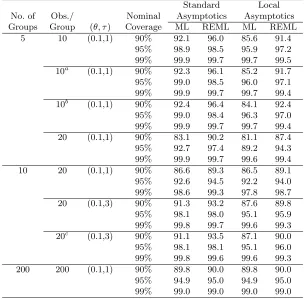
[image:12.612.116.420.255.554.2]variance of the elements of u, is the parameter of interest. None of the intervals performed particularly well, though it was generally the case that the coverage accuracy was best for the likelihood-based intervals (12) and (13) and worst for the central intervals (4) and (10). In addition, the coverage of intervals based on the adjusted profile log-likelihoods tended to be more accurate than those based on the usual profile log-likelihood, though not exclusively so. Among the adjusted profile log-likelihoods discussed in Section 2, the profiled REML log-likelihood was generally the most accurate and so we present results only for this adjustment of the profile log-likelihood here. Finally, the coverage of intervals based on the local asymptotics tended to be more accurate than those based on the standard asymptotics, though again not exclusively so.
Table 1: Coverage accuracy of likelihood-based intervals (100,000 simulations).
Standard Local
No. of Obs./ Nominal Asymptotics Asymptotics
Groups Group (θ, τ) Coverage ML R EML ML R EML
5 10 (0.1,1) 90% 92.1 96.0 85.6 91.4
95% 98.9 98.5 95.9 97.2
99% 99.9 99.7 99.7 99.5
10a (0.1,1) 90% 92.3 96.1 85.2 91.7
95% 99.0 98.5 96.0 97.1
99% 99.9 99.7 99.7 99.4
10b (0.1,1) 90% 92.4 96.4 84.1 92.4
95% 99.0 98.4 96.3 97.0
99% 99.9 99.7 99.7 99.4
20 (0.1,1) 90% 83.1 90.2 81.1 87.4
95% 92.7 97.4 89.2 94.3
99% 99.9 99.7 99.6 99.4
10 20 (0.1,1) 90% 86.6 89.3 86.5 89.1
95% 92.6 94.5 92.2 94.0
99% 98.6 99.3 97.8 98.7
20 (0.1,3) 90% 91.3 93.2 87.6 89.8
95% 98.1 98.0 95.1 95.9
99% 99.8 99.7 99.6 99.3
20c (0.1,3) 90% 91.1 93.5 87.1 90.0
95% 98.1 98.1 95.1 96.0
99% 99.8 99.6 99.6 99.3
200 200 (0.1,1) 90% 89.8 90.0 89.8 90.0
95% 94.9 95.0 94.9 95.0
99% 99.0 99.0 99.0 99.0
aGroup Sizes = (6,6,10,14,14);bGroup Sizes = (2,6,10,14,18); cGroup Sizes = (10,10,15,15,20,20,25,25,30,30).
W(θ), based on either the unadjusted profile log-likelihood (ML) or the profiled REML log-likelihood (REML). The intervals based on local asymptotics tend to have lower coverage than the corresponding intervals based on the standard asymp-totics, indicating that the local asymptotic approximation generally will not im-prove the coverage accuracy if the standard approximation produces undercoverage. Typically, however, in cases with small variance components, methods based on the standard asymptotics are seen to overcover, so that local asymptotic methods offer an improvement in coverage accuracy. For instance, at the nominal 90% level the ML intervals typically perform quite well with the standard asymptotics. On the other hand, both the likelihood and REML intervals are typically conservative at the nominal 95% and 99% levels so the coverage is improved by using the local asymptotic approximation. Generally, however, the differences in performance are not substantial. Furthermore, we note that results (not reported here) on the cov-erage accuracy of interval (13) based on the profiled REML log-likelihood show that its coverage accuracy is typically slightly superior to the more intuitively appealing intervals derived from (12). However, interval (13) does not perform substantially better, and does occasionally perform worse, than interval (12). Moreover, for the smaller sample sizes, (13) led to null intervals in an appreciable number of samples. In particular, for the balanced case of c1 = 5 and m = 10 with (θ, τ) = (0.1,1),
[image:13.612.106.432.305.563.2]there were about 3% of samples which led to empty 95% confidence intervals, and nearly 5% of samples which led to empty 90% confidence intervals.
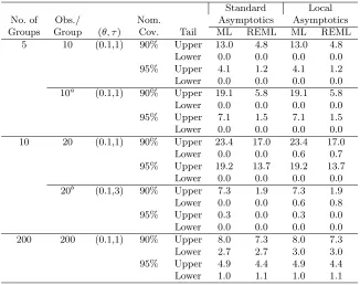
Table 2: Upper and lower non-coverage probability of central intervals (100,000 simulations).
Standard Local
No. of Obs./ Nom. Asymptotics Asymptotics
Groups Group (θ, τ) Cov. Tail ML REML ML REML
5 10 (0.1,1) 90% Upper 13.0 4.8 13.0 4.8
Lower 0.0 0.0 0.0 0.0
95% Upper 4.1 1.2 4.1 1.2
Lower 0.0 0.0 0.0 0.0
10a (0.1,1) 90% Upper 19.1 5.8 19.1 5.8
Lower 0.0 0.0 0.0 0.0
95% Upper 7.1 1.5 7.1 1.5
Lower 0.0 0.0 0.0 0.0
10 20 (0.1,1) 90% Upper 23.4 17.0 23.4 17.0
Lower 0.0 0.0 0.6 0.7
95% Upper 19.2 13.7 19.2 13.7
Lower 0.0 0.0 0.0 0.0
20b (0.1,3) 90% Upper 7.3 1.9 7.3 1.9
Lower 0.0 0.0 0.6 0.8
95% Upper 0.3 0.0 0.3 0.0
Lower 0.0 0.0 0.0 0.0
200 200 (0.1,1) 90% Upper 8.0 7.3 8.0 7.3
Lower 2.7 2.7 3.0 3.0
95% Upper 4.9 4.4 4.9 4.4
Lower 1.0 1.1 1.0 1.1
aGroup Sizes = (6,6,10,14,14),bGroup Sizes = (10,10,15,15,20,20,25,25,30,30).
the usual interval (4) while the local asymptotic approximation leads to the interval (10). These intervals exhibit extremely poor, and decidedly asymmetric, coverage accuracy, even for the “large sample” case ofc1= 200 andm= 200. Moreover, the use of local asymptotic approximations has little impact on the coverage accuracy. This outcome is not altogether surprising. When the probability associated with point mass at the origin in the local asymptotic approximation exceeds 0.025, symmetric non-coverage is impossible and the only non-coverage occurs in the upper tail. In general, extremely large samples are needed before the asymptotics apply for these intervals. This is largely due to treating the standard error as constant inθ. Confidence intervals based on the Wald test use essentially the same construction but treat the standard error as a function ofθ and, although we do not present the results here, generally perform nearly as well as the likelihood-based intervals presented in Table 1. The general conclusion from Table 2 is that straightforward application of asymptotics associated with parameter estimators is not a very reliable or accurate method for constructing confidence intervals.
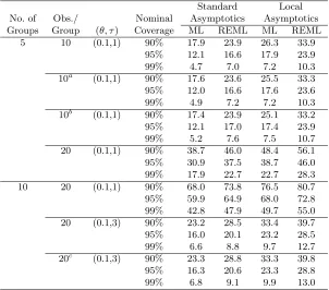
[image:14.612.118.420.266.532.2]Finally, the power of likelihood ratio and REML tests against the null hypoth-esis that θ = 0 using the two asymptotic approximations is explored in Table 3.
Table 3: Power againstH0:θ= 0 of likelihood-based tests (100,000
simulations).
Standard Local
No. of Obs./ Nominal Asymptotics Asymptotics
Groups Group (θ, τ) Coverage ML R EML ML R EML
5 10 (0.1,1) 90% 17.9 23.9 26.3 33.9
95% 12.1 16.6 17.9 23.9
99% 4.7 7.0 7.2 10.3
10a (0.1,1) 90% 17.6 23.6 25.5 33.3
95% 12.0 16.6 17.6 23.6
99% 4.9 7.2 7.2 10.3
10b (0.1,1) 90% 17.4 23.9 25.1 33.2
95% 12.1 17.0 17.4 23.9
99% 5.2 7.6 7.5 10.7
20 (0.1,1) 90% 38.7 46.0 48.4 56.1
95% 30.9 37.5 38.7 46.0
99% 17.9 22.7 22.7 28.3
10 20 (0.1,1) 90% 68.0 73.8 76.5 80.7
95% 59.9 64.9 68.0 72.8
99% 42.8 47.9 49.7 55.0
20 (0.1,3) 90% 23.2 28.5 33.4 39.7
95% 16.0 20.1 23.2 28.5
99% 6.6 8.8 9.7 12.7
20c (0.1,3) 90% 23.3 28.8 33.3 39.8
95% 16.3 20.6 23.3 28.8
99% 6.8 9.1 9.9 13.0
aGroup Sizes = (6,6,10,14,14),bGroup Sizes = (2,6,10,14,18), cGroup Sizes = (10,10,15,15,20,20,25,25,30,30)
likelihood ratio tests, so that the REML test based on the local asymptotic ap-proximation has the highest power in these comparisons. The power is related to the length of the confidence intervals presented in Table 1 with higher power being associated with shorter intervals. Of course, there are other aspects of the interval methods which affect the power, but Table 3 does provide an indirect exploration of the lengths of the intervals.
The above results show that further research on the problem of setting con-fidence intervals for small components of variance is needed. In the meanwhile, our tentative suggestion is that intervals be constructed from the REML version of the likelihood ratio test with the local asymptotic approximation to its sampling distribution, as this method seems to have the best overall combination of coverage and power properties.
REFERENCES
O. E. Barndorff-Nielsen (1983). On a formula for the distribution of the maximum likelihood estimator. Biometrika, 70, 343–365.
O. E. Barndorff-Nielsen (1994). Adjusted versions of profile likelihood and directed likelihood, and extended likelihood. Journal of the Royal Statistical Society Series B, 56, 125–140.
O. E. Barndorff-Nielsen & S. R. Chamberlin (1992). Stable and invariant adjusted likelihood roots. Technical Report. Department of Theoretical Statistics, Aarhus University, Aarhus, Denmark.
R. K. Burdick & F. A. Graybill (1988). The present status of confidence interval estima-tion on variance components in balanced and unbalanced random models. Commu-nications in Statistics: Theory and Methods (Special Issue on the Analysis of the Unbalanced Mixed Model), 17, 1165–1195.
H. Chernoff (1954). On the distribution of the likelihood ratio. The Annals of Mathe-matical Statistics, 25, 573–578.
D. R. Cox & N. Reid (1987). Parameter orthogonality and approximate conditional inference (with discussion). Journal of the Royal Statistical Society Series B, 49, 1–39.
N. Cressie & S. N. Lahiri (1993). The asymptotic distribution of REML estimators.
Journal of Multivariate Analysis, 45, 217–233.
T. J. DiCiccio, M. A. Martin, S. E. Stern & G. A. Young (1996). Information bias and adjusted profile likelihoods. Journal of the Royal Statistical Society Series B, 58, 198–203.
T. J. DiCiccio & S. E. Stern (1993). An adjustment to profile likelihood based on observed information. Technical Report. Department of Statistics, Stanford Uni-versity, Stanford, CA.
Z. Feng & C. E. McCulloch (1992). Statistical inference using maximum likelihood estimation and the generalized likelihood ratio when the true parameter is on the boundary of the parameter space. Statistics and Probability Letters, 13, 325–332. D. Firth (1993). Bias reduction of maximum likelihood estimators. Biometrika, 80,
27–38.
J. K. Ghosh & R. Mukerjee (1994). Adjusted versus conditional likelihood: power properties and Bartlett-type adjustments. Journal of the Royal Statistical Society Series B, 56, 185–188.
V. P. Godambe (1960). An optimum property of regular maximum likelihood estimation.
M. G. Kenward & J. H. Roger (1997). Small sample inference for fixed effects from restricted maximum likelihood. Biometrics, 53, 983–997.
A. Y. C. Kuk (1995). Asymptotically unbiased estimation in generalized linear models with random effects. Journal of the Royal Statistical Society Series B, 57, 395–407. B. Levin & F. Kong (1990). Bartlett’s bias correction to the profile score function is a
saddlepoint correction. Biometrika, 77, 219–221.
K.-Y. Liang (1987). Estimating functions and approximate conditional likelihood. Bio-metrika, 74, 695–702.
P. McCullagh & R. J. Tibshirani (1990). A simple method for the adjustment of profile likelihoods. Journal of the Royal Statistical Society Series B, 52, 325–344.
P. A. P. Moran (1971). Maximum likelihood estimation in non-standard conditions.
Proceedings of the Cambridge Philosophical Society, 70, 441–450.
H. D. Patterson & R. Thompson (1971). Recovery of inter-block information when block sizes are unequal. Biometrika, 58, 545–554.
H. D. Patterson & R. Thompson (1974). Maximum likelihood estimation of components of variance. Proceedings of the 8th International Biometric Conference, 197–207. A. M. Richardson & A. H. Welsh (1994). Asymptotic properties of restricted maximum
likelihood (REML) estimates for hierarchical mixed linear models. The Australian Journal of Statistics, 36, 31–43.
A. M. Richardson & A. H. Welsh (1996). Covariate screening in mixed linear models.
Journal of Multivariate Analysis, 58, 27–54.
S. R. Searle, G. Casella & C. E. McCulloch (1992). Variance Components. Wiley, New York.
S. G. Self & K.-Y. Liang (1987). Asymptotic properties of maximum likelihood ratio tests under non-standard conditions. Journal of the American Statistical Association, 82, 605–610.
S. E. Stern (1997). A second-order adjustment to the profile likelihood in the case of a multidimensional parameter of interest. Journal of the Royal Statistical Society Series B, 59, 653–665.
S. J. Welham & R. Thompson (1997). A likelihood ratio test for fixed model terms using residual maximum likelihood. Journal of the Royal Statistical Society Series B, 59, 701–714.
J. S. Williams (1962). A confidence interval for variance components. Biometrika, 49, 278–281.
Received 28 January 1999 Steven E.Stern
Accepted 28 October 1999 [email protected]
Department of Statistics and Econometrics The Australian National University Canberra, ACT Australia, 0200
A. H.Welsh [email protected]