doi:10.4236/ijcns.2010.36067 Published Online June 2010 (http://www.SciRP.org/journal/ijcns/).
Performances of Chaos Coded Modulation Schemes Based
on Mod-MAP Mapping and High Dimensional LDPC
Based Mod-MAP Mapping with Belief Propagation
Decoding
Naim Khodor, Jean-Pierre Cances, Vahid Meghdadi, Raymond Quere University of Limoges, XLIM-Department, Limoges, France
E-mail: {naim.khodor, cances, frmeghdadi, raymond.quere}@ensil.unilim.fr Received February 5,2010; revised March 11,2010; accepted April 15,2010
Abstract
In this paper, we propose to generalize the coding schemes first proposed by Kozic et al. to high spectral ef-ficient modulation schemes. We study at first Chaos Coded Modulation based on the use of small dimen-sional modulo-MAP encoding process and we give a solution to study the distance spectrum of such coding schemes to accurately predict their performances. However, the obtained performances are quite poor. To improve them, we use then a high dimensional modulo-MAP mapping process similar to the low-density generator-matrix codes (LDGM) introduced by Kozic et al. The main difference with their work is that we use an encoding and decoding process on GF (2m) which enables to obtain better performances while pre-serving a quite simple decoding algorithm when we use the Extended Min-Sum (EMS) algorithm of De-clercq & Fossorier.
Keywords:Chaos Coded Modulation, Expectation Maximization, Gaussian or Rayleigh Mixtures, Low-Density Parity-Check (LDPC), Low-Density Generator-Matrix (LDGM), Factor Graph, Extended Min-Sum (EMS)
1. Introduction
Since the pioneering work of Frey in 1993 [1], chaotic communications has been an important topic in digital communications. Due to their extreme sensitivity to ini-tial conditions which, for example, facilitates theoreti-cally the separation of merging paths in a trellis based code, these systems have also been considered as good potential candidates for channel encoding [2-7]. This explains why chaotic modulations and channel encoders derived from chaotic systems have been extensively studied in the open literature. According to us, there are mainly two types of chaos based channel encoders de-pending on the size of the transmitted alphabet. The first kind of chaos based channel encoders includes non-linear generators which transmit binary messages and benefit from the correlation between successive transmitted bits to obtain some coding gain. Due to the poor spectral ef-ficiency, it is rather easy to optimize this kind of codes to obtain a non-null free distance and to obtain reasonable good performances, i.e., codes that outperform un-coded
working at a joint waveform and coding level, can be efficient in additive white Gaussian noise channels [21- 23]. These promising works on the AWGN channel have been recently further extended by Escribano & al in the case of Rayleigh flat fading channels [24].
In this work, we use Chaos Coded Modulation designs of S. Kozic [25,26] and we optimize them using the tance spectrum. We find that the distance spectrum dis-tribution can be good approximated by Rayleigh prob-ability distribution function (pdf). Using this optimiza-tion step, we can optimize their structures. Furthermore we show that using a high dimensional modulo-MAP mapping process we are able to considerably improve the performances of this kind of schemes and to obtain per-forming codes. This principle is related to the former work of Kozic & Hasler in [27]. In their work, low-den-sity generator-matrix (LDGM) codes are used as natural interleave in front of mappings to signal constellation. That is why this kind of code can be assumed as particu-lar kind of BICM. However, the chaotic map is used as joint coding (interleaving) and modulation, and thus, the complete system is a single code. The framework of it-erative decoding is based on factor graphs, which is a graphical representation of codes. LDPC and LDGM linear block codes have a very simple graphical repre-sentation called Tanner graph. However, for nonlinear codes, the graphical representation is not so simple, and this may be the reason why the large potential of nonlin-ear codes is not yet exploited. The main difference with their work is that we use an encoding and decoding process on GF (2m) which enables to obtain better
per-formances while preserving a relative simple decoding algorithm when we use the Extended Min-Sum (EMS) algorithm of Declercq & Fossorier [28]. The contribu-tions of our paper are thus the following ones.
Detailed study of the distance spectra of the chaos based encoders and characterization of their distribution.
New encoding and decoding process based on the use of graph factorization and the use of Belief Propagation (BP) algorithm over high order Galois fields GF (2m).
The rest of the paper is organized as follows. In Sec-tion 2, we give the basic principles for the chaos coded modulation schemes proposed by S. Kozic. We propose to approximate the distance distribution with some usual laws such as the Rayleigh one. In Section 3, we show the high dimensional coding process based on LDPC over GF(2m); simulation results are provided which
demon-strate the outstanding performances of these structures. Concluding remarks are eventually given in Section 4.
2. Chaos Coded Modulation Scheme,
Distance Spectrum Study
2.1. Chaotic Coder Structure
We consider the Chaos-Coded modulation scheme of
Figure 1. This scheme was originally given by S.
Kozic in his PhD works [26]. The scheme of Figure 1.
can be represented by means of a convolutional coder of rate = 1/(n.(Q + 1)), where at each time step k, one bit bk enters the coder and a vector of (Q+1) bits v = [vQ,vQ-1,…,v0]T is produced. The signal constellation is
realized by a weighted sum of vectors 2-i. A(Q-i+1) mod
(1) where A is some matrix which optimizes the dis-tance spectrum of the code. This mapping, due to the modulus operation, is a highly non-linear operation and serves as a chaos generator. Henceforth, we have a system which combines a convolutional coder with a multi-dimensional mapping in the same way as Multi- level Trellis Coded Modulation (M-TCM). The corres- ponding convolutional coder is classically described by:
, , 1 ,0
v ( )
( ) . ... .
( )
Q i
i i Q i Q
D
h D t t D t D b D
i (1)
S. Kozic defines several possible matrices T= {ti,j} in his work which give good performances:
1 0 0 0 1 0 0 0
shift
T
tent
1 0 1 0 1 0 0 0
e shift
T
1 0 0 1 1 0 1 1
T
Concerning, the choice of the matrix A, we can write the transmitted vector at the output of the modulator:
1
1
0 1
2 2
a
a
a
Q Q
i Q i i
k i i
i i Q
x A v D v D
mod 1 (2)Before transmitting xk on the channel propagation
medium, we modulate each of its components in NRZ-BPSK, i.e., : xk → 2 xk -1.
Rather than a global optimization algorithm which should look for the convolutional coder together with the mapping process, we choose to fix a convolutional coder structure and then we work on the mapping process by using a particular form of matrix A. We found that the choice Ti,j= Tshift for i = j and Ti,j=Ttent
for i ≠ j enables to obtain a large set of performing non-linear mapping with A. For example, in the case n
= 2, using this choice for matrices T, we are looking for matrices A with the following structure:
21
1 1
1
a
A .
and we optimize the choice of a21 using the distance
spectrum. In the case, n = 3, we use matrix form:
21 31 32 1 1 1
1 1 1
a a a
x
KT0Q
T1Q
TQQ
bk bk-n+1
T01
T11
TQ1
T00
T10
TQ0 bk-Qn bk-(Q+1)n+1
+
1
2 . AQ
1 2. 2 AQ
1 0
[image:3.595.147.450.87.342.2]2 Q .A
Figure 1. Trellis chaos-coded modulation encoder.
The choice of the remaining parameters ai,j is done using the distance spectrum of the code. The state of the coder is defined by vector Sk:
Sk= [bk,…,bk-n,…bk-Qn,…,bk-(Q+1).n+1]T (3)
Concerning the choice of Q, it’s clear that the Vi- terbi decoding algorithm is rapidly limited by the com-plexity in the number of states which is equal to 2n.(Q+1). Practically, the number n(Q + 1) should not exceed 12 which correspond to 4096 states. For n = 2, this gives a maximum value of Q equal to 5, and for n = 3, this gives a maximum value of Q equal to 3. The choice of
Qa, is more complicated and is related to the chaotic behaviour of the coder.
2.2. Spectrum Distance Analysis
In order to optimize the coders, we study their distance spectrum. To do this, we have to determine the trajec-tories in the trellis which start with a common state Si = Si* and evolve in disjoint paths for (L-1) time steps
and then merge again into the same state Sk = Sk* not
necessarily equal to Si. This kind of trajectory in the
trellis defines a loop and the loop is characterized by its initial state Si, its final state Sk and its length L. The
distance of corresponding codewords belonging to the two competing paths in the loop is:
2 1
2 , ,
1 i k
L
L S S m m
m
d
x x* (4)The problem of the computation of (4) is that, unlike
linear codes when we can choose a reference path equal to a all zero sequence, due to the non-linear mapping, we have to test all the possible transmitted sequence for a given loop length together with all the possible starting states. Hence, the distance spectrum computation prob-lem is of non polynomial complexity and in straightfor-ward manner requires the inspection of all possible initial conditions and all possible controlled trajecto-ries. For example, there are 2n.(Q+1).2nL different
con-trolled trajectories of length L. In order to compute the distance spectrum with a reasonable complexity while keeping a sufficient accuracy, we form all the possible pair of sequences starting from a given state and both converging towards an other state after L steps with L
belonging to the interval [Qn + 1, n.(Q + m)], i.e. the length of the loop varies from Qn+1 (the constraint length of the code plus one) to to n.(Q + m) (we limit practically the search to m = 2 or 3 in our case due to the computation burden). We have partitioned the dis-tance spectrum into subsets by distinguishing error events which entail one error bit, error events which entail two error bits, error events which entail three error bits and so on. In practice, we limit our search to error events which entail five maximum error bits since simulation results evidenced that it was sufficient to obtain accurate upper bounds for the BER.
We obtain for example with matrices: Ti,j=Tshift for i = j and Ti,j=Ttent (i.e.n = 2) for i≠j and a21= 8, Q
= Qa = 3, the distance spectrum illustrated on Figure 2.
distribu-tion with the following probability density funcdistribu-tion: 2 2
( ) / 2. 2
( )
( ) .
( ) 0
j j x j C j j j C x
f x e x
x f x (5)
[image:4.595.72.275.531.701.2]For example, with the distance spectrum plotted on
Figure 2, we calculate parameters μj and σj2 to obtain
the best fitting between the pdf of the distance spec-trum and fc(x,mj,σj2) we obtain with classical MMSE
technique: μj σj2 6.7. This corresponds to a
mini-mum free distance of the coder equal to dfree 6.7. We have developed an original EM (Expectation-Maximization) algorithm to obtain the approximated Rayleigh distribu-tion of the distance spectrum as a mixture of Rayleigh laws. The mixture of Rayleigh laws can be written as:
2 2
( ) / 2. 2 1 2 1 ( ) ( ) . . . ( , ) n n J x n C n n n J
n n n
n
x
f x e
(6)where (μn,σn2) represents a Rayleigh law of
parame-ters: μn and σn2. The Maximum Likelihood (ML)
re-search algorithm to find:πn,μn, σn2 can be summarized
as:
1
1
: 1
2
: 1 1 1
ˆ arg max log ( )
arg max log . ( ; , )
J j j J j j n J
j i j j
i j p
(7)where ψ (x,μ,σ2) denotes the value of a Rayleigh law of
parameters μ,σ2 at x. For a fixed number of mixtures J,
based on the observations: ,i = 1,…,n, the pa-rameters j,mj,j,j=1,…,J can be estimated using the EM (Expectation Maximization) algorithm. The algorithm proceeds in two steps:
E-step: Compute
Figure 2. Distance spectrum of the chaos coded modulation.
( )
( )
( ) i log ( )
i
Q E p X (8)
M-step: solve
( 1)i arg max Q( ( )i)
j
(9)
Define the following hidden data Z = zi, i = 1,…, n
where zi is a J-dimensional indicator vectoring such that:
2 ,
1, ( , )
0 ,
i j
i j
if R m
z otherwise
(10)
The complete data is then X (,Z), we have : ,
2 1 1
( , ) n J . ( ; , zi j j i j j i j
p R m
Z (11)
The log-likelihood function of the complete data is then given by:
, 1 1 2 2 , 2 1 1log , .log
. log log
2
n J
i j j
i j
n J i j
i j i j j
i j j
p Z z
z C
(12)where C is a constant. The E-step can then be calculated as follows:
'
( ') log ( , )
Q E p Z
2, 2
1 1
( ')
ˆ . log log 2 log
2
n J i j
i j j i j j
i j j
Q
z C
We have:
' ' ' , , ,' '2 ' ' '2 ' 1
ˆ , 1
( ; , ).
( ; , ).
i j i j i j i
i j j j J
i l l l l
z E z P z
m m
(13)The M-step is calculated as follows. To obtain j, we have:
'
, 1
( , ) 1 ˆ
0 j .n i j, 1,...,
i j Q z j n
J (14)
To obtain μj, we have: '
, 2
1
( , ) 0
( )
1
ˆ .[ ] 0, 1,...,
j n
i j
i j
i i j j
Q m m z j m J
2 2, 2 2
1
( )
ˆ .[ ] 0, 1,...,
.( )
n
j i j
i j
i j i j
...,J
2 2 2
, ,
1 1
2
, ,
1 1
2 2
, ,
1 1
ˆ . ˆ .( 2. . ), 1,
ˆ . 2. . ˆ .
ˆ ˆ
. . , 1,...,
n n
i j j i j i j i j
i i
n n
i j i j i j i
i i
n n
j i j i j j
i i
z z m m j
z m z
m z z j J
(15)
To obtain {σj} we have the set of equations: '
2
, 3
1
( , ) 0
( )
2
ˆ .[ ] 0, 1,...,
j n
i j i j
i j j
Q
m
z j J
J
2 2
, ,
1 1
ˆ ˆ
2. .j n i j n i j.( i j) , 1,...,
i i
z z m j
(16)2 ,
2 1
, 1
ˆ .( )
, 1,...,
ˆ 2.
n
i j i j i
j n
i j i
z m
j z
J (17) (17) The set of Equations (16) and (17) is a set of coupled non-linear equations and we use the optimization toolbox with the function fsolve to solve (16-17) at each maximi-zation step.The set of Equations (16) and (17) is a set of coupled non-linear equations and we use the optimization toolbox with the function fsolve to solve (16-17) at each maximi-zation step.
2.3. Performances over AWGN Channels 2.3. Performances over AWGN Channels
To end this part, we give some BER results on AWGN channels, using the optimization obtained by the distance spectrum computation to find good modulation parame-ters. Due to a lack of place we only give simulation re-sults. For n = 2, we obtain the following result on Figure 3.
To end this part, we give some BER results on AWGN channels, using the optimization obtained by the distance spectrum computation to find good modulation parame-ters. Due to a lack of place we only give simulation re-sults. For n = 2, we obtain the following result on Figure 3.
The chaotic coder outperforms un-coded BPSK at high SNR’s due to good asymptotic properties with a moder-ate high free distance. The weakness of this kind of code is their poor coding rate. There are several solutions to improve this. The first is to make input bits enter the coder by groups of k bits. In this case, the coding rate becomes equal to: k/n.(Q + 1).
The chaotic coder outperforms un-coded BPSK at high SNR’s due to good asymptotic properties with a moder-ate high free distance. The weakness of this kind of code is their poor coding rate. There are several solutions to improve this. The first is to make input bits enter the coder by groups of k bits. In this case, the coding rate becomes equal to: k/n.(Q + 1).
However, this considerably reduces the correlation degree between consecutive states and renders the trellis non-binary. We found that the penalty encountered by this method too much important (using k = 2 results in 4
However, this considerably reduces the correlation degree between consecutive states and renders the trellis non-binary. We found that the penalty encountered by this method too much important (using k = 2 results in 4 dB losses compared to k = 1) so we prefer using punc-turing to increase the coding rate of our proposed coders. We added the case of punctured codes on Figure 4 with
the best puncturing patterns we found for rate 8/7 and 4/3.
dB losses compared to k = 1) so we prefer using punc-turing to increase the coding rate of our proposed coders. We added the case of punctured codes on Figure 4 with
the best puncturing patterns we found for rate 8/7 and 4/3.
The conclusions are nearly the same, considering the case n = 3 as it is illustrated on Figure 4.
The conclusions are nearly the same, considering the case n = 3 as it is illustrated on Figure 4.
With a free distance equal to 13 for the optimized code With a free distance equal to 13 for the optimized code
BER
Figure 3. Performances of Trellis Chaos-Coded Modulation over AWGN channels for n = 2, Q = 3.
with rate 1/9, the punctured codes (9/7) are able to out perform un-coded BPSK at high SNR’s. To complete this overview of BER performances over AWGN channels, it is important to say that using the approximate pdf’s of the distance spectrum, we are able to accurately predict the BER at high’s SNR’s. To complete the results, we give on Figure 12 the best performances we found with n = 3, Q = 3 (i.e. the number of states is 4096).
In fact, as it is expected, increasing the quantization level for a given dimensionality n, entails some losses. Compared to Figure 4, the loss in terms of SNR for a
[image:5.595.308.540.83.256.2]BER of 10-4, 10-5 is approximately 1 dB on
Figure 5 and
punctured codes are unable to outperform un-coded BPSK.
It is clear that the obtained performances remain poor.
BER
[image:5.595.306.540.494.680.2]binary/q-ary converter is then used to obtain vectors
dk+i-Q= (dk+i-Q(1), dk+i-Q(2),…, dk+i-Q(n-1), dk+i-Q(n))T of q-ary
symbols: di(p), p = 1,2,…,n belonging to the alphabet: A =
(0,1,…,q-1). Each obtained vector dk+i-Q is then
multi-plied by a sparse low-density based matrix AQ-I and
weighted by a factor 2-(i+1) then, the new resulting
en-coding vectors are added to obtain the vector:
BER ( 1)
0
2 . . mod(
Q
i Q i
k k i Q
i
q
z A d ).
Finally, to obtain a chaotic trajectory we add the vec-tor: 2-(Q+1).(A-I).e with: e [1, 1,…, 1]T. This yields to the
following equation:
( 1) -0
2
2 . . . mod
2
Q Q
i Q i
k k i Q
i
q
[image:6.595.58.284.79.254.2]x A d p (19)
Figure 5. Performances of optimized Trellis Chaos-Coded Modulation over AWGN channels for n = 3, Q = 3 (4096 states).
With: p=2-Q.(A-I).e=K.(A-I).e.
The coding sequence at the output of the modulator is then equal to: x = (x1, x2,…, xk,…).The relation (19) is
called the high-dimensional expansion associated with the chaotic system (18). Another way to represent the encoding rule is to use the following equation:
To increase them, we propose to generalize the non-linear output mapping to matrices A of high-dimension.
3. High Dimensional LDPC Based
Mod-MAP Mapping with B.P Decoding
xk1 2. .A xkmodq2 .(Q dk11/ 2. ) mode q (20)The relation (20) is simpler than (19) to better under-stand the encoding algorithm; however Equation (19) is more suitable for the factorization of the factor graph. The rule (20) represents a dynamical system controlled with stochastic perturbations of small amplitudes 2-Q
which constitute the input signal. It is obvious that as: Q
→+∞, the small amplitudes vanish and the output signal vector becomes the chaotic state.
3.1. The Encoding Process
The generalized mod-MAP function is written as:
1 2. . mod
k k q
x A x (18)
where xkistheinput vector of size n and A is a n × n
ma-trix with elements belonging to alphabet: A = (0, 1,…,
q-1) with q = 2m since we take here: q =2m for the
con-sidered Galois-field GF(q). The encoding scheme is drawn on Figure 6. The binary streams b = (b1, b2,…, bk,…) are
grouped into vector vector bk+i–Q of size: n.m = n.m with m denoting the spectral efficiency we want to use in the encoding-decoding process. Hence, we can write:
bk+i–Q= (bk+i–Q(1), bk+i–Q(2),…, bk+i–Q(nm-1), bk+i–Q(nm))T. A
It is important to note that the decoding of a LDPC over GF(q) implies that we use a systematic form for the encoding process. It’s the case here since b = (b1, b2,…,
bk,…) is the systematic part and x = (x1, x2,…, xk,…) is
the redundancy check part. We have of course a overall coding rate of 0.5 because the systematic part and the redundancy check part have the same dimension.
( 1)
2 Q .(A- I e).
-1
2 .AQmod(2 )m
-2Q.Amod(2 )m - 1 2Q .
n
I
(nm1) k Q b
( 1) 1 m n k b
(nm 1) k
b (1)
k
b Binary to q-ary
Binary to q-ary
Binary to q-ary
(1) 1 k b
(1) k Q b
(2) k b
(2) 1 k b
(2) k Q b
(nm) k b
( ) 1 m n k b
(nm) k Q b
[image:6.595.125.475.568.694.2]x
k3.2. Factor Graphs
To explain how the factorization can be efficiently im-plemented it is convenient to represent a function with a factor graph. Once a factor graph has been found it is straightforward to use the BP (Belief Propagation) algo-rithm to determine the marginal of a multivariate func-tion. For linear block codes the factor graph of the code becomes a Tanner graph. Of course, in our case due to the use of a non-linear encoding process, finding this graph is a much more complicated task. In fact as Kozic demonstrated in [27], there are mainly two possible solu-tions to obtain it here. The first one consists in using the party-check equation given by Equation (20). The second one is the consequence of the high-dimensional expan-sion associated with Equation (19). The first solution is not appropriate since it would imply to obtain informa-tion about bk from the soft information about the states xk
which constitute the graph of variable and check nodes and dk is multiplied by a small value: 2-Q. Hence the
re-liability about information concerning bk would be small
in this case. Hence, the second solution is the only trac-table one. However, it is important to avoid the use of successive power of A in the graph factorization. This is due to the fact that short cycles of length four appear when we use for example A2 in a factor graph even if A
does not exhibit short length cycles.
The graph factorization may be expressed in the fol-lowing way: it comprises mainly three steps. The first one is related directly to the scheme of Figure 6 and
concerns the computation of xkgiven dk+i-Q it will be
named high-order expansion graph. The second one concerns the LDPC code contained in each matrix A, it will be named GF(q) LDPC graph and finally the third one concerns the way the input bits slide to constitute a new vector to be encoded. This mechanism is related to the convolutional encoder behaviour and will be named convolutional graph.
The high-order expansion graph constitutes the main original part and it can be obtained as follows. We con-sider at first an indicator function of high dimensional
q-ary expansion:
( 1) -0
( , ,..., )
1, if 2 . . . mod
2 0, otherwise
k k k Q Q
i Q i
k k i Q
i g q q
x d d
x A d p (21)
We can use then additional variables μi,jdefined as:
( 1) ,
0
2 . mod
Q
Q
k i Q i
i q
x p
Of course, we have the relationship: μi,j+1 = A. μi,j.mod
qwith:μi,0 = 2-(i+1)dk+i-Q. With these variables, function g
becomes a function only of variables: μi,j. To keep on
factorizing g we introduce functions gi,j+1 defined as : , 1 ,
, 1 , 1 ,
1, if . mod
( , )
0, otherwise
i j i j i j i j i j
q g
A (22)
and g0:
0 0, 1, 1
( 1) ,
0
( , , ,...)
1, if 2 . mod
0, otherwise
k Q Q
Q
Q k i Q i
i g q
x x p The corresponding factorization of g is given by:
0 0 0
(.) . (.)
Q Q i ij i j
g g g
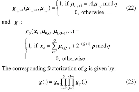
(23)The factorization is drawn below on Figure 7.
It is possible to further factorize the class of functions:
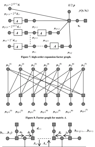
gi,j+1. The variables at the left side of Equation (22) will
be named the checks and the variables on the right side will be considered as the noisy symbols. We define similarly as in the case of LDPC codes: (l) = {m:alm ≠
0} the set of noisy symbols that participate in the check l. In the same way, we define: (m) = {l:alm≠ 0} the set of checks that depend on the noisy symbol m. In this case (22) can be written as:
( ) ( )
, 1 ,
( )
. mod , [1, ] [1,
l m
i j lm i j
m l
a q m l n
n]
(24)
Let:
( ) ( )
, 1 ,
( ) ( )
, 1
1, if . mod
0, otherwise
l m
i j lm i j
l m l
i j
a q
g
(25)
The symbols on Figure 7 correspond either to variable
nodes (circle on the figure) or check nodes (square on the figure). The symbolise decoding of the complete chaotic trajectory is given by:
. . 0,1 0 1 1 1 arg max , ,..., ,..., , .k i Q
k i Q
M Q
j j
d j
d
j j j Q
j j Q j j j
p p g p p
x
y xx d d
d d x x d
(26)
The quantity ≈dk+1-Q means summation over all
com-ponents except: dk+1-Q. Furthermore, the graph of matrix A is classically those of a LDPC code over GF(q) and is drawn on Figure 8.
The shift register and the binary q-ary conversion set operation, which represent transition state from time j to time j + 1 can be given by the indicator function: gc=
p(xj+1|xj,dj+1). The state at time j + 1 depends on the
sym-bol sequence: dj+1,…,dj+1-Q, and it can be computed using
[image:7.595.305.544.96.254.2] [image:7.595.330.531.521.597.2]μQ-2,0 = 2-(Q-1) dk-2 μQ-1,1
μQ-2,1
μ0,1
μ0,Q-1
A
μ0,Q
μQ-2,2
K/2 p
xk p(yk/xk)
A
A
μQ,0 = 2-(Q+1) dk
μQ-1,0 = 2-Qdk-1
A
μ0,0 = 2-1 dk-Q
[image:8.595.140.465.71.570.2]A
Figure 7. high-order expansion factor graph.
μi,j(1) μi,j(2) μi,j(3) μi,j(4) μi,j(5) μi,j(6) μi,j(7)
μi,j+1(1) μi,j+1(2) μi,j+1(3) μi,j+1(4) μi,j+1(5) μi,j+1(6) μi,j+1
(7)
Figure 8. Factor graph for matrix A.
dk+1
Λin
(b0,…,b-Q) αk δk βk γk ( bM+Q+1,…,bM+1)
Λex
Figure 9. Factor graph of the complete chaotic code.
about symbol: dj+1. Using together factorization gc and
factorization of the high-order expansion of Figure 7, the
decoding problem of (26) can be presented with the fac-tor graph of Figure 9. This graph takes into account the
shift register process which includes new incoming bits into the encoding process and consists of two recursions: forward and backward recursions as in the well known BCJR algorithm.
The parameters αk, βk, γkand δk are defined in the same
way as in [27] except that we work at symbol level for the computation of αk,βk,γk and δk.
Note that since the main difference with the scheme proposed by Kozic, et al. in [27] consists in the use of a non-binary encoding scheme, we have to transform a priori probabilities on bits to a priori probabilities in symbols. This is done using the formula:
( ) ( ) ( ) ( )
(1) (2) . ( )
. ( ) 1
[ ( , ,..., ) ]
1
j j
e k i Q k i Q
j j
e k i Q k i Q
m T
k i Q k i Q k i Q k i Q
b b
m
b b
j
P b b b
e e
d
)
where designs the log-likelihood ratio
cor-responding to bit: bk+i-Q(j). For the complementary
prob-lem, i.e. when we have to express the log-likelihood ratio of bit bk+i-Q(j) from the log-likelihood ratios of
corre-sponding symbols, we have:
( )
( j e bk i Q
( ) ( ) ( 1).
( ) ( ) ( 1).
( )
: 1
( 1). )
(
: 0
( ) log
j e k i Q
j j m k
k i Q k i Q
j e k i Q
j j m k
k i Q k i Q
d d b
j m k
e k i Q d
d b
e
b
e
))
m
(28)
where, obviously, corresponds to the log-
likelihood ratio of symbol:
( ) ( j e dk i Q
( )j [ (j 1).m 1, (j 1).m 2,..., (j 1).m ] k i Q k i Q k i Q k i Q d b b b .
3.3. Iterative Decoding
The main steps of the iterative decoding are the same as those of [27] except for the use of a non-binary generator matrix A. The decoding of LDPC codes over GF(q) has been an extensive research topic recently. Among all the decoding algorithms, we choose the Extended Min-Sum (EMS) Algorithm in the log-domain proposed by De-clercq and Fossorier [28] since it exhibits a good trade- off between performance and complexity. To explain the main principles we use the following notations. A parity node in a LDPC code over GF(q) with q= 2m represents
the following parity equation:
1
( ). ( ) 0 mod ( )
c
d
k k
k
h x i x m x
(29)where m(x) in the modulo operator is a degree m -1 primitive polynomial of GF(q). Equation (29) expresses that the variable nodes needed to perform the BP algo-rithm on a parity node are the codeword symbols multi-plied by non-zeros values of the parity matrix H. The corresponding transformation of the graph is performed by adding variable nodes corresponding to the
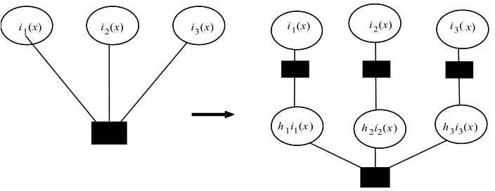
multipli-cation of the codeword symbols ik(x) by their associated nonzero H values and is illustrated on Figure 10.
The function node that connects the two variable nodes ik(x) and hk(x). ik(x) performs a permutation of the message values. The permutation that is used to update the message corresponds to the multiplication of the ten-sor indices by hk(x).from node ik(x) to node hk(x). ik(x) and to the division of the indices by hk(x) the other way. With this transformation of the factor graph, the parity node update is indeed a convolution of all incoming messages as in the binary case.
To express the EMS algorithm, we use the following notations for the messages in the graph. Let {Vpv} v = 1,…,dv be the set of messages entering a variable node of degree dv, and {Uvp}v = 1,…,dv be the output messages for this variable node. The index ‘p.v’ indicates that the message comes from a permutation node to a variable node, and ‘v.p’ is for the other direction. We define similarly the messages {Upc} c = 1,…,dc (resp. {Vpc} c = 1,…,dc) at the input (resp. output) of a degree dc check node. The EMS algorithm works in the log-domain and uses reduced configuration sets to simplify the computa-tional task. We define then:
1
[image:9.595.121.473.565.701.2]1 1
[ ,..., ]
[ ... ] log ( ,..., ) {0,1}
[0,...,0]
m m
m m
U i i
U i i i i
U
(30)
As the log-density-ratio (LDR) representations of the messages. In the considered q-ary case, the message is composed of q -1 nonzero LDR values. The purpose of the EMS algorithm is to simplify the parity check node update by selecting only the most probable configuration sets of q-ary symbols which get involved in the parity check equations. To do that, we start by selecting in each incoming message Upc the nq largest values (we will take nq fixed in our simulation results for simplicity rea-sons) that we denote: ( )kc
pc
u , kc = 1,…,nq. We use the following notation for the associated field element:
( )kc ( )
c x
, so that we have:
i2(x)
i1(x) i3(x) i1(x) i2(x) i3(x)
i1
h1 (x) h2i2(x) h3i3(x)
1
( ) ( )
( ) ( )
Prob( ( ). ( ) ( )) log
Prob( ( ). ( ) 0) [ ... ] c c c c m k
k c c c
pc
c c
k k
pc c c
h x i x x u
h x i x U (31)
With these largest values, we build the following set of configurations:
1 1
1
1 ( )
( )
1 1 1
Conf ( )
[ ( ),..., dc ( )] : [ ,..., ] 1,..., c c dc q d k k T k d n
x x k k n
k q
(32) any vector of dc-1 field elements in this set is called a
configuration. The set Conf(nq) corresponds to the set of configurations built from the nq largest probabilities in each incoming message. Its cardinality is:
1
Conf ( ) dc
q q
n n .
we need to assign a reliability to each configuration; we take as in [28]:
( ) 1... 1
( ) c
c k k c c d L u
.The initialization of the decoder is achieved with the channel log-likelihoods defined as: L[i1,…,im].
The EMS proceeds in three steps as given below:
Sum-step: variable node update for a degree dv node:
v v v 1,v 1,..., d tp p t
U L V t d
v (33)or: v
1 1
v 1 1
v 1,v
[ ,..., ] [ ,..., ]
[ ,..., ] ( ,..., ) {0,1}
tp m m
d
m
p m m
t
U i i L i i
V i i i i
Permutation-step: from variable to check nodes:
1
v 1 1
[ ,..., ]
[ ,..., ] ( ,..., ) {0,1} with ( ) ( ). ( )
pc m
m
p m m
U i i
U j j i i i x h x j x
(34)
The permutation step from check to variable nodes is
performed using: 1 .
( )
h x
P
Message update: for a degree dc check node:
From the dc-1 incoming messagesUpc, build the sets:
( ) Conf ( )( ,1) Conf ( )( , )
dc dc dc
i x i x i x p c
S q n n , Then:
1
( ) 1
[ ,..., ]
max ( ) ( ,..., ) {0,1}
c c cp
k idc x c cp
d p d d
m
S k d d
V i i
L i i
(35) With: ( ) 1 ( ) 1 Conf ( , )
{ Conf ( , ) : ( ). ( ) ( ) 0}
dc
c c c c
i x p c
d k
k p c d d c
c
n n
n n h x i x x
Post-processing: 1 1 1[ ,..., ] [ ,..., ] [0,...,0] ( ,..., ) {0,1} , 1,...,
cp m cp m cp
m
m c
V i i V i i V
i i c d
(36)
3.4. Simulation Results
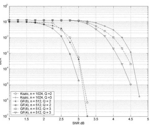
We give here some simulation results to show the per-formance of the proposed scheme. Since the target com-parison is the work of Kozic & al [27], we use their re-sults as benchmark for our proposed system. In his work, Kozic plots the obtained BER results for n = 512 and 1024 as the size of the vector input bits together with Q = 2 or 3 and a random sparse matrix with weight ρ= 3 or 6 on each column. We take each time the best perform-ances he obtained.
Using the same size of input blocks, we have to choose the desired spectral efficiency. Due to the heavy computational task, we only take here: q = 4 and q = 8;
i.e.; we work with GF(4) and GF(8) with spectral effi-ciencies respectively equal to 2 and 3 bits/s/Hz. The ob-tained results are drawn on Figure 11 for block size 512
and on Figure 12 with block size 1024.
One notices that the performances of our GF(q) LDPC codes of size 512 are quite similar to those of Vucetic & al for size 1024 and, using block size of length 1024, our designs outperform clearly those of Vucetic & al. The SNR gain for block size 1024 is approximately equal to 0.5 dB for Q = 2 and for GF(8) and becomes 0.75 dB for
Q = 2 and for GF(4). The improvement is slightly better in the case Q = 3 since we obtain gains of 1.0 dB for
GF(8) and 1.5 dB for GF(4). This result is not really surprising since many authors have shown that LDPC codes over GF(q) exhibit better performances than their counterparts on GF(2). One can notice that the slopes i.e.; the diversity gain are the same each time in the waterfall region. A more detailed study should be done to deter-mine the starting point SNR of the waterfall region with the EXIT-CHART curves.
4. Conclusions
Figure 11. BER performances for chaos based LDPC codes over GF(q); block-length size equal to: 512.
Figure 12. BER performances for chaos based LDPC codes over GF(q); block-length size equal to: 1024.
hence we can optimize the BER performances of such schemes. In the case where we use high dimensional sparse matrices for the MOD-MAP mapping, we can use a decoding process similar to those of LDPC codes. When we compare our obtained results with those of the former literature we noticed that, working on GF(q) en-ables to obtain significant gains of approximately 1. dB. This encouraging result entails the necessity to further optimize the design to reduce the hardware complexity. In fact, despite the use of the Extended Min-Sum algo-rithm, the obtained coding structure remains of prohibi-tive complexity.
5. References
[1] D. R. Frey, “Chaotic Digital Encoding: An Approach to
Secure Communication,” IEEE Transactions on Circuits and Systems II, Vol. 40, No. 10, 1993, pp. 660-666. [2] A. Layec, “Développement de modèles de CAO pour la
simulation système des systèmes de communication. Application aux communications chaotiques,” Ph.D. Thesis, Xlim University of Limoges, 2006.
[3] F. J. Escribano, L. Lopez, M. A. F. Sanjuan, “Evaluation of Channel Coding and Decoding Algorithms Using Discrete Chaotic Maps,” Chaos, American Institute of Physics, No. 16, 2006, pp. 1054-1500.
[4] I. P. Marino, L. Lopez, M. A. F. Sanjuan, “Channel Coding in Communications Using Chaos,” Physics Letters Elsevier Science, Vol. 295, No. 4, 2002, pp. 185-191.
[image:11.595.178.420.315.507.2]Chaos,” Physical Review Letters American Physical Society, Vol. 79, No. 19, pp. 3787-3790.
[6] T. Schimming and M. Hasler, “Coded Modulation Based On Controlled 1-D and 2-D Piecewise Linear Chaotic Maps,” IEEE International Symposium on Circuits and Systems (ISCAS), pp. 762-765.
[7] B. Chen and G. W. Wornel, “Analog Error Correcting Codes Based on Chaotical Dynamical Systems,” IEEE
Transactions on Communications, Vol. 46, No. 7, pp.
881-890.
[8] T. Erseghe and N. Bramante, “Pseudo Chaotic Encoding Applied to Ultra-Wide-Band Impulse Radio,” IEEE Vehicular Technology Conference, Vancouver, September 2002, pp. 1711-1715.
[9] J. Lee, C. Lee and D. B. Williams, “Secure Communi- cations Using Chaos,” IEEE Globecom’95, Singapore, November 1995, pp. 1183-1187.
[10] J. Lee, S. Choi and D. Hong, “Secure Communications Using a Chaos System in a Mobile Channel,” IEEE Globecom’98, Sydney, November 1998. pp. 2520-2525. [11] C. Lee and D. B. Williams, “A Noise Reduction Method
for Chaotic Signals,” 44th IEEE Acoustic, Sensor and Signal Processing Conference (ICASSP), Detroit, May 1995, pp. 1348-1351.
[12] A. M. Guidi, “Turbo and LDPC Coding for the AWGN and Space-Time Channel,” Ph.D. Thesis, University of South Australia, South Australia, June 2006.
[13] S. A. Barbulescu, A. Guidi and S. S. Pietrobon, “Chaotic Turbo Codes,” IEEE Conference International Sympo- sium on Information Theory (ISIT), June 2000, p. 123. [14] X. L. Zhou, J. B. Liu, W. T. Song and H. W. Luo,
“Chaotic Turbo Codes in Secure Communications,”
Conference EUROCON’2001, International Conference
on Trends in Communications, July 2001, pp. 199-201. [15] A. Abel and W. Schwarz, “Chaos Communications-
Principles, Schemes, and System Analysis,” Proceedings of the IEEE, Vol. 90, No. 5, May 2002, pp. 691-710. [16] W. M. Tam, F. C. M. Lau and C. K. Tse, “Digital
Communications with Chaos,” Elsevier, Oxford, 2007.
[17] S. Kozic, K. Oshima and T. Schimming, “How to Repair CSK Using Small Perturbation Control-Case Study and Performance Analysis,” Proceedings of ECCTD, Krakow, August 2003.
[18] Y. S. Lau, Z. M. Hussain, “A New Approach in Chaos Shift Keying for Secure Communication,” Proceedings of the third International Conference on Information Tech- nology and Applications (ICITA’05), Sydney, pp. 630- 633.
[19] H. Dedieu, M. P. Kennedy and M. Hasler, “Chaos Shift Keying: Modulation and Demodulation of a Chaotic Carrier Using Self-Synchronizing Chua’s Circuits,” IEEE Transactions on Circuits and Systems II: Analog and Digital Signal Processing, Vol. 40, No. 10, 1993, pp. 634-642.
[20] J. Schweitzer, “The Performance of Chaos Shift Keying: Synchronization Versus Symbolic Backtracking,” Pro- ceedings of the IEEE International Symposium on Cir- cuits and Systems (ISCAS), Monterey, 1998, pp. 469- 472.
[21] F. J. Escribano, L. Lopez and M. A. F. Sanjuan, “Parallel Concatenated Chaos Coded Modulations,” IEEE Con- ference 15th International Conference on Software, Tele- communications and Computer Networks, Softcom, 2007. [22] F. J. Escribano, L. Lopez and M. A. F. Sanjuan,
“Iteratively Decoding Chaos Encoded Binary Signals,”
Proceedings of the Eighth International Symposium on Signal Processing and its Applications, 2005, Sydney, August 2005, pp. 275-278.
[23] S. Kozic, T. Schimming and M. Hasler, “Controlled One- and Multidimensional Modulations Using Chaotic Maps,”
IEEE Transactions on Circuits and Systems I: Regular Papers, Vol. 53, No. 9, September 2006, pp. 2048-2059. [24] F. J. Escribano, L. Lopez and M. A. F. Sanjuan,