Nonlinear Control of an Induction Motor Using a
Reduced-Order Extended Sliding Mode Observer for
Rotor Flux and Speed Sensorless Estimation
Olivier Asseu1, Michel Abaka Kouacou1*, Theophile Roch Ori1, Zié Yéo 1, Malandon Koffi1, Xuefang Lin-Shi2
1Département Génie Electrique et Electronique, Institut National Polytechnique Houphouët Boigny
(INP HB), BP 1093 Yamoussoukro Côte d’Ivoire
2Université de Lyon, AMPERE, INSA Lyon, CNRS UMR
5005, Villeurbanne 69621, France
E-mail: [email protected]
Received July 13, 2010; revised August 19, 2010; accepted August 21, 2010
Abstract
This article proposes an innovative strategy to the problem of non-linear estimation of states for electrical machine systems. This method allows the estimation of variables that are difficult to access or that are sim-ply impossible to measure. Thus, as compared with a full-order sliding mode observer, in order to reduce the execution time of the estimation, a reduced-order discrete-time Extended sliding mode observer is proposed for on-line estimation of rotor flux, speed and rotor resistance in an induction motor using a robust feedback linearization control. Simulations results on Matlab-Simulink environment for a 1.8 kW induction motor are presented to prove the effectiveness and high robustness of the proposed nonlinear control and observer against modeling uncertainty and measurement noise.
Keywords:Robust Nonlinear Control, Induction Motor, Reduced-Order Extended Sliding Mode Observers, Parameter Estimation
1. Introduction
The induction motors (IM) become very popular for mo-tion control applicamo-tions due to its reasonable cost, sim-ple and reliable construction. However, the control of IM is proved very difficult since the dynamic systems are non linear, the electric rotor variables are not usually measurable or the transducers are expensive (such as torque, seed, flux transducers) and the physical parame-ters are often imprecisely known or variable. For in-stance, the rotor resistance drifts with the temperature of the rotor current frequency.
This naturally structure of non-linear and multivariable state of IM models induces the use of the non-linear control methods and in particular the robust feedback linearization strategy [1-3] to permit a decoupling, assure a good dy-namic performance and stability of the IM.
However, a variation of the rotor resistance can induce a state-space “coupling” which can induce a degradation of the system. In order to achieve better dynamic per-formance, an on-line estimation of rotor fluxes, speed and rotor resistance is necessary. An approach proposed
in [4,5] to estimate with success the state variables in an IM is the use of the full-order Sliding Mode Observer (SMO). This latter, built from the dynamic model of the IM by adding corrector gains with switching terms, is used to provide not only the unmeasurable state variable estimation (rotor fluxes and speed) but also the estima-tion of the measurable parameters (stator currents). How-ever the determination of the measurable parameters es-timation imposes some eses-timation algorithms very long and usually sophisticated with an increase of the compu-tational volume. Therefore, in order to reduce the accu-racy and the computation rate of the estimation algo-rithms, the measured parameters estimation is not neces-sary.
Thus a Reduced-Order Discrete-Time Extended Slid-ing Mode Observer (RDESMO) for the IM is presented in this paper to solve only and specially the problem of the unmeasurable parameters estimation (rotor fluxes, speed and rotor time constant).
discrete-time Extended Sliding Mode Observer (ESMO) is developed in Section 3. Section 4 describes the simu-lation results carried out on a 1.8 kW IM drive system. Finally, conclusions are summarized in Section 5.
2. Induction Motor Model and Robust
Feedback
Control
By assuming that the saturation of the magnetic parts and the hysteresis phenomenon are neglected, the classical dynamic model of the IM in a (d, q) synchronous refer-ence frame can be described by [6]:
; . . . . ds s qs qs s qs qs s ds ds s ds dt d I R V dt d I R V qs s qr r m qs ds s dr r m ds I L L L I L L L . . . . (1.a) dr ds r m m s dr ds I I L L L L ; qr qs r m m s qr qs I I L L L L (1.b) The load mechanical equation is:
where . m( . . )
r
r em r em dr qs qr ds
r L d
J f
C C C p
p dt J L
(1.c) The application of (1.a) to (1.c) returns a system of fifth-order non-linear differential equation, with as state variables the stator currents (Ids, Iqs), the rotor fluxes (dr,
qr) and the rotor pulsation (r): ( ) .
c c c c
x f x g u where
xc = [Ids Iqsdrqrr]t, u = [Vds Vqs]t
2 . . . . . . . . ( ) . . . . ; . . . . . .( . . ) . . . 1 0 . 1 0 . 0 0 0 0
ds s qs r dr r qr
s ds qs r dr r qr
c c r m ds r dr sl qr
r m qs sl dr r qr
m
dr qs qr ds r r
r
s
s c
f x L
L
L p f
p C
L J J J
L L g 0 0 (2) 2 m
1 1 1
; ( ) (1 ). ;
L 1
; = 1
. .
r r r
r s
m s r
T T
L L L
Moreover, by choosing a rotating reference frame (d, q) so that the direction of axe d is always coincident with the direction of the rotor flux representative vector (field orientation), it is well known that this rotor field orienta-tion in a rotating synchronous reference frame realizes:
dr = r = Constant and qr = 0 (3) Thus the dynamic model of the IM, completed with the output equation, can be rewritten as:
( ) .
x f x g u ; y =[h1(x) h2(x)]t = [r r ]t with x = [Ids Iqsrr]t, u = [Vds Vqs]t
0 0 0 0 . 1 0 0 . 1 ; . . . . . . . . . . . . . . . . . ) ( 2 s s r r qs r r m r r ds m r r r qs ds s r r qs s ds L L g J f C J p J L L p L x f (4)
From the expressions (2) and (3), one can write:
qs r r m em qs mr sl r mr r ds r mr L L p C dt d . . . . .
with mr r m I L
(5) This relation (5) shows that the dynamic model of the IM can be represented as a non-linear function of the rotor time constant. A variation of this parameter can induce, for the IM, a lack of field orientation, perform-ance and stability. Thus, to preserve the reliability, ro-bustness performance and stability of the system under parameters variation (in particular the rotor time constant variations) and disturbances, we can uses a robust feed-back linearization strategy to regulate the motor states.As a matter of fact, we can see that the system (4) has relative degree r1 = r2 = 2 and can be transformed into a
z1 = h1(x); z2 = Lf h1(x); z3 = h2(x); z4 = Lf h2(x);
the feedback linearization control having the fol-lowing form:
1 2
1 1 2 1 1 1
2
1 2 2 2 2 2
( ) ( ) ( )
( ) ( ) ( )
g f g f f
g f g f f
L L h x L L h x v L h x u
L L h x L L h x v L h x
where v1 and v2 are the new inputs of the obtained
de-coupled systems
and two robust controllers C(s) to provide a good regulation and convergence of the rotor flux (r) and speed (r). On the other hand, in order to im-pose after a closed loop a second order dynamic behaviour defined by H(s), the controller C(s) can be chosen by [8]:
1
2 0
2 0
2
0 0
( ). ( ) 1
( ) ; ( ) ;
1 ( ) (1 )
1 ( )
2 1
1
J s H s
C s J s
J s t s
H s
s s
(6)
where the real t0is an adjusting positive parameter. The block diagram structure for the control of (r, r) is as follows:
Furthermore, as the control of an IM generally required the knowledge of the instantaneous flux of the rotor that is not measurable, a full-order SMO built from the model (2) by adding corrector gains with switching terms is widely used [7,9] with success for on-line estimation at one and the same time of rotor time constant, fluxes, currents or speed. The equivalent value of the switching function de-pends on the current errors given by the difference between the estimated currents to their real or measured values. However, as the currents are already measurable, their es-timated values are not therefore necessary.
Thus in the next section, in order to reduce the execu-tion time of the observaexecu-tion with respect to the rotor time constant variations, a RDESMO is proposed to provide only the unmeasurable parameters estimation (rotor fluxes, rotor time constant and speed). And the switching term of this reduced observer will be only function of the measurable parameters (voltage, currents…).
3. Reduced-Order Discrete-Time Extended
Sliding Mode Observer
3.1 Reduced-Order Sliding Mode Observer
Let us consider the dynamic model of the IM given by
the system (2). Assume that among the state variable, the stator currents (Ids, Iqs) are measurable, therefore their on-line estimation is not necessary. Thus from the ex-pression (2), in order to estimate only the rotor flux (dr, qr) and speed (r), a reduced dimensional state vector defined by Xr= [drqrr]T =[x1 x2 x3], T can be intro-duced. The corresponding reduced-order state space equation becomes:
( ) ( ), ( )
r r r
x t J x t t
Where (t) = [Ids, Iqs]T is the new input.
rsl 11 slr 22 r2
1 2 3
. . . .
( ), ( ) . . .
. .( . . ) . .
.
r m ds
r r m qs
m
qs ds r
r
x ω x L I J x t t ω x x L .I
L p f
p I x I x C x
L J J J
(7) The fact that the state vector only consists of the rotor flux and speed offers an advantage namely the reduction of the computational volume and complexity. Thus the rotor flux and speed can be more easily and rapidly estimated. Denote xˆ1,xˆ2and xˆ3the estimates of the fluxes dr, qr andr. The Reduced-order SMO is a copy of the model (7) by adding corrector gains with switching terms:
1 r 1 sl 2 r m ds 1 s 2 sl 1 r 2 r m qs 2 s
2
3 qs 1 ds 2 3 3 s
ˆ .ˆ .ˆ . . .
ˆ .ˆ .ˆ . . .
ˆ . .( .ˆ . )ˆ . . .
. m
r r
x σ x ω x σ L I Γ Ι
x ω x σ x σ L I Γ Ι
L p f
x p I x I x C x Γ Ι
L J J J
(8)
where 1, 2 and 3 are the observer gains. The switch-ing “Is” is defined as
1 1
2 2
1 3 3
sign( )
; . ;
sign( )
ˆ
. .
ˆ
. .
s r
r r
s s
I S M Z
s s
x M
x
(9)
where Z~r is a function depending on the parameters measurements (stator currents, voltages…).
Setting x x x ˆ , the estimation error dynamics is given by:
1 1 sl 2 1
2 sl 1 r 2 2 s
2
3 1 2 3 3
. . .
. . .
. .( . . ) . .
.
r s
m
qs ds s
r
x σ x ω x Γ Ι
x ω x σ x Γ Ι
L f
x p x I x I x Γ Ι
L J J
(10)
With the following observer gain matrices given by the expression (11), the estimation error
~x1,~x2,~x3
con-- + C(s)
Feedback algorithm (rRef , rRef)
Motor model
verges to zero.
1 2
3 2 2
0 . ;
0
. .
. .
. .
r sl
sl r
m qs m ds
r r
r
n r
n L I L I
p p
L J L J
(11)
where r and n are positive adjusting parameters which play a critical role in the stability and the velocity of the observer convergence.
3.2. Reduced-Order Extended Sliding Mode Observer
In order to estimate the rotor time constant, a reduced dimensional extended state vector defined by Xre= [dr qrrr]T =[x1 x2 x3 x4] T has been introduced with r =
Rr/Lr. The corresponding reduced-order extended state space equation becomes:
( ) ( ), ( )
re re re
x t J x t t where
4 1 sl 2 4
sl 1 4 2 4
2
1 2 3
. . . .
. . . .
( ), ( )
. .( . . ) . .
.
m ds m qs
re r m
qs ds r
r
x x ω x x L I
ω x x x x L I
J x t t L p f
p I x I x C x
L J J J
(12) where presents the slow variation of r. The pro-posed Reduced-order ESMO is:
1 4 1 sl 2 4 1
2 sl 1 4 2 4 2
2
3 1 2 3 3
4 4
ˆ ˆ ˆ. .ˆ ˆ . . .
ˆ .ˆ ˆ ˆ. ˆ . . .
ˆ . .( .ˆ . )ˆ . .ˆ .
.
ˆ .
m ds s
m qs s
m
qs ds r s
r s
x x x ω x x L I Γ Ι
x ω x x x x L I Γ Ι
L p f
x p I x I x C x Γ Ι
L J J J
x Γ Ι
(13)
where is, 1, 2 and 3 are respectively defined by (9) and (11).
To determine observer gain 4, it can be supposed that the observation errors of the fluxes converge to zero. The estimation errors of the fluxes xi x xi ˆi 0 (i = 1,2) are then given by:
4 1 4 1 2 4 1
1 4 2 4 2 4 2
ˆ ˆ
0 . . . .
ˆ ˆ
0 . . . .
sl m ds s
sl m qs s
x x x x x L I x I
x x x x x L I x I
(14)
By replacing the expressions of 1 and 2 in (14), the es-timation error dynamics of the rotor time constant is given by:
1 1
1 1
4 4 4 4 4
2 2
ˆ . 1
. . . .
ˆ . m ds s
m qs
L I x
x
x I x
L I x
x r
We can see that this error dynamics is locally and expo-nentially stable by chosen:
1 4
2
ˆ .
. . . .
ˆ .
T m ds m qs
L I x
m r
L I x
with m > 0 (15)
The parameter m is adjusted with respect to rotor time constant estimation.
Finally, from the expressions (11) and (15), it can be seen that there are three positive adjusting gains: r, n and
m which play a critical role in the stability and the veloc-ity of the observer convergence. These three adjusting parameters must be chosen so that the reduced observer satisfies robustness properties, global or local stability, good accuracy and considerable rapidity.
In order to implement the reduced-order ESMO algo-rithm in a DSP for real-time applications, the corre-sponding reduced-dimension state space equation de-fined in (12) must be discretized using Euler approxima-tion (1st order). Thus the new discrete-time varying model represented by a function depending on the stator current is given by:
( 1) ( ) . ( ) ( ) . ( ), ( )
( ) ( )
re
re re e J re re e re
re re
x k x k T L x k x k T q x k v k
y k x k
with
2
qs ds r
( ), ( )
( ). ( ) ( ). ( ) ( ). . ( )
( ). ( ) ( ). ( ) ( ). . ( )
;
. . ( ). ( ) ( ). ( ) . . ( )
. 0
re
r dr sl qr r m ds
sl dr r qr r m qs
m
dr qr r
r
q x k v k
k k k k k L k
k k k k k L k
L p f
p I k k I k k C k
L J J J
(16) where k means the kth sampling time, i.e.t = k.Te with Te the adequate sampling period chosen without failing the stability and the accuracy of the discrete-time model. The proposed RDESMO can be defined by the following equation:
ˆre( 1) ˆre( ) e. ˆre( ), ( ) ( ). ( )s
x k x k T q x k v k G k I k (17) where the prediction vector is:
( 1) ( ) . ( ), ( )
re re e re
x k x k T q x k v k
with x kre( ) dr( )k qr( )k r( )k r( )k T
1 2 1 2
sign( ( ))
( ) with
sign( ( ))
( )
. ( ). ( 1) ( )
s
e
s k I k
s k s k
S T M k Z k s k
(18)
where
l l
ˆ ( ) ( ) ( )
ˆ ( ) ( )
r s
s r
k k M k
k k
,
ˆ ( 1) ( 1) ( 1)
ˆ ( 1) ( 1)
rd rd
rq rq
z k z k z k
z k z k
Let us introduce the measure vector
zr(k+1) = [zrd(k+1), zrq(k+1)]T written as follows:
r r
( 1) ( 1) ( ) . ( ). ( )
rd d d e s qr
z k k k T k k and
qr
( 1) ( 1) ( ) . ( ). ( )
rq qr e s dr
z k k k T k k
From the electrical Equation (1.a) of the IM, an ap-proximate (1st order) discrete-time relation of the fluxes is given by:
. .
( 1) ( ) . ( ) ( 1) ( ) . ( ). ( )
. . .
( 1) ( ) . ( ) ( 1) ( ) . ( ). ( )
e r s r
rd ds s ds ds ds e s qs
m m
e r s r
rq qs s qs qs qs e s ds
m m
T L L .L
z k V k R I k I k I k T k I k
L L
T L L L
z k V k R I k I k I k T k I k
L L
and
ˆ ( 1) ( 1) ( ) ( ). ( )
ˆ ( 1) ( 1) ( ) . ( ). ( )
rd dr dr e s qr
rq qr qr e s dr
z k k k T . k k
z k k k T k k
(19)
The proposed gain matrix representation G(k), de-duced from the continuous case given by (11) and (15),
can be defined as follows (discrete-time approach):
1 2
2 2
3 4
ˆ
. ( ) . ( )
( )
. ( ) .ˆ ( )
( )
.
( ) .
. .
( ) . .
. .
( )
ˆ ˆ
.( . . ( ) ( )) .( . . ( ) ( ))
e r e sl
e sl e r
m qs
r m ds
e e
r r
e m ds dr e m qs qr
r T k T k
k
T k r T k
k
L I
G k L I
T p
k T p
L J L J
k
T m L I k k T m L I k k
(20)
Once the fluxes are estimated, it is easy to deduce the estimated torque defined by:
ˆ ( ) . m ˆ ( ). ( ) ˆ ( ). ( )
em dr qs qr ds
r
L
C k p k k k k L
(21)
4. Simulation Results
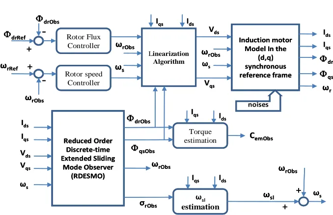
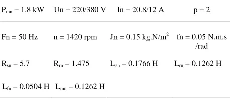
In order to verify the feasibility of the proposed RDESMO, the simulation on SIMULINK from Mathwork has been carried out for a 1.8 kW induction motor controlled with a robust linearization via feedback algorithm (Figure 1). The nominal parameters of the induction motor are given in the Table 1.
The RDESMO is implanted in a S_function using C language. In order to evaluate its performances and ef-fectiveness, the comparisons between the observed state variables and the simulated ones have been realized for several operating conditions with the presence of about 15% noise on the simulated currents (Ids, Iqs) or speed. Thus, using a sampling period Te = 1 ms, the simulations are realized at first in the nominal case with the nominal parameters of the induction motor (Table 1) and then, in the second case, with 50% variation of the nominal rotor
time constant (r = 1.5 rn) in order to verify the rotor time constant tracking and flux estimation.
Figure 2 and Figure 3 show the simulation results for a step input of the rotor speed and flux. One can see that in both nominal (Figures 2(a), 2(c)) or non-nominal (Figures 3(a’), 3(c’)) cases, the estimated values of fluxes and torque converge very well to their simulated values.
The observed fluxes (Figure 2(a)) indicate the good orientation (dr is constant and qr converges to zero) which is due to a favorable rotor time constant estimation (Figures 2(b), 3(b’)). The estimated torque (Figure 2(c)) is in good agreement with the simulated value.
Once the fluxes are estimated, we can deduce the al-gorithm of the feedback linearization control (Figure 1). The waveforms show the good uncoupling between the rotor flux and the speed because a step variation in dr (Figure 2(a) and Figure 3(a’)) can not generate a speed
r change (Figure 2(d) and Figure 3(d’)). Thus the field orientation and the synthesis of robust linearization and decoupling control are well verified.
ωsl
estimation Rotor Flux
Controller
Rotor speed Controller
Induction motor Model In the
(d,q)
synchronous reference frame
Reduced Order
Discrete‐time Extended Sliding
Mode Observer (RDESMO)
‐
+
+
‐
drRef
ωrRef
ωs Vds Vqs Ids Iqs
σrObs
drObs
qsObs
Ids Iqs
Ids Iqs
dr qs
Ids Iqs
+ +
ωr
ωsl
Torque estimation
noises
CemObs
ωs ωs
Vqs
Vds
ωs
Linearization Algorithm
Ids Iqs
drObs
ωrObs ωrObs
ωrObs
ωrObs
ωrObs
ωsl
estimation Rotor Flux
Controller
Rotor speed Controller
Induction motor Model In the
(d,q)
synchronous reference frame
Reduced Order
Discrete‐time Extended Sliding
Mode Observer (RDESMO)
‐
+
+
‐
drRef
ωrRef
ωs Vds Vqs Ids Iqs
σrObs
drObs
qsObs
Ids Iqs
Ids Iqs
dr qs
Ids Iqs
+ +
ωr
ωsl
Torque estimation
noises
CemObs
ωs ωs
Vqs
Vds
ωs
Linearization Algorithm
Ids Iqs
drObs
ωrObs ωrObs
ωrObs
ωrObs
[image:6.595.126.465.69.288.2]ωrObs
Figure 1. Simulation scheme of the system.
Figure 2. (a, b, c, d): Nominal case (Rr = Rrn). Figure 3. (a’, b’, c’, d’): Non nominal case (Rr = 1.5Rrn).
[image:6.595.267.530.326.686.2]
Table 1. Nominal parameters of the induction motor.
Pmn = 1.8 kW Un = 220/380 V In = 20.8/12 A p = 2
Fn = 50 Hz n = 1420 rpm Jn = 0.15 kg.N/m2 fn = 0.05 N.m.s
/rad
Rsn = 5.7 Rrn = 1.475 Lsn = 0.1766 H Lrn = 0.1262 H
Lfn = 0.0504 H Lmn = 0.1262 H
5. Conclusions
We have shown in this paper that a robust feedback lin-earization strategy and RDESMO are used to permit a regulation and observation for the Induction motor states in order to assure a good dynamic performance and stabil-ity of the global system. In order to reduce the observation execution time, this RDESMO, based on the full -order SMO principle, permit only and specially for the recon-struction of the parameters non measurable in an IM (the fluxes, speed and the rotor time constant estimation).
The interesting simulation results obtained on the in-duction motor show the effectiveness, the convergence and the stability of this robust decoupling control and RDESMO against rotor resistance variations, measured noises and load. Thus, in order to validate the robustness of this non-linear control and RDESMO, Experimental results on a testing bench for a 1.8 kW induction motor will be present in the next research project.
6. References
[1] D. I. Krein, I. J. Ha and M. S. Ko, “Control of Induction Motors via Feedback Linearization with Input-Output Decoupling,” International Journal of Control, Vol. 51, No. 4, 1989, p. 863-883.
[2] K. B. Mohanty, N. K. De and A. Routray, “Sensorless Control of a Linearized and Decoupled Induction Motor Drive,” National Power Systems Conference, NPSC, Kharag-pur, India, December 2002, pp. 46-49.
[3] R. Yazdanpanah, J. Soltani and G. R. A. Markadeh, “Nonlinear Torque and Stator Flux Controller for Induc-tion Motor Drive Based on Adaptive Input-Output Feed-back Linearization and Sliding Mode Control,” Energy
Conversion and management, Vol. 49, No. 4, 2008, pp. 541-550.
[4] P. A. Bogdan and A. Keyhani, “Sliding-Mode Flux Ob-server with Online Rotor Parameter Estimation for Induc-tion Motors,” IEEE Transactions on Industrial
Electron-ics, Vol. 54, No. 2, April 2007, pp. 716-723.
[5] A. Derdiyok, “Speed-Sensorless Control of Induction Motor Using a Continuous Control Approach of Slid-ing-Mode and Flux Observer,” IEEE Transactions on
Industrial Electronics, Vol. 52, No. 4, August 2005, pp. 1170-1176.
[6] D. F. Bernard and L. Jean-Paul, “Identification et observation des actionneurs électriques,” Vol. 1 & 2, Hermes, Paris, 2007.
[7] O. Asseu, Z. Yeo, M. Koffi, X. Lin-Shi, C. T. Haba and G. L. Loum, “Robust Decoupling Control and Extended Sliding Mode Observer for an Induction Motor,” News
-Phys Chem, Vol. 48, July 2009, pp. 1-8.
[8] J. C. Doyle, B. A. Francis and A. R. Tannenbaum, “Feed-back Control Theory,” Maxwell MacMillan Internat, New York, 1992.
[9] M. Tursini, R. Petrella and F. Parasiliti, “Adaptive Slid-ing Mode Observer for Speed Sensorless Control of In-duction Motors,” IEEE Transactions on Industry
Applica-tions, Vol. 36, No. 5, September/October 2000, pp. 1380 -1387.
Nomenclature
Cem, Cl: Electromagnetic and load torques, N.m. f: friction coefficient, Nm.s/rad.
Ids, Iqs, Imr: Stationary frame (d,q)-axis stator currents
and rotor magnetizing current, A.
J: inertia, kg.m2.
Lr, Ls, Lm, Lf: rotor, stator, mutual and leakage
induct-ances, H.
p: pole pair number.
Rs, Rr: stator and rotor referred resistance, .
Te, Tr, Ts: sampling period, rotor and stator time
con-stant (Tr = Lr/Rr = 1/σr; Ts = Ls/Rs), s.
Vds, Vqs: Stationary frame d- and q-axis stator voltage, V.
dr, qr: d-q components of rotor fluxes, Wb.
ds, qs: d-q components of stator fluxes, Wb.
s, r, sl : stator, rotor and slip pulsation (or speed),