Abstract
Mummert, Craig, The development of a machine vision system to measure the shape of a sweetpotato root (Under the direction of Dr Michael D. Boyette, Dr Larry F Stikeleather, and Dr. M. K. Ramasubramanian)
The objective of this project is to develop and investigate whether a machine vision system can quantitatively describe the physical characteristics of a sweetpotato and then produce a unique number that is a more accurate descriptor of the root. Machine vision has been shown to accurately measure the size and shape of various agricultural commodities by mapping their surfaces. This map can then be used to describe the characteristics of the object. For this study a system was developed to rotate the root in front of a CCD imaging device that maps the entire surface of the sweetpotato.
The development of a machine vision system to measure the shape of a
sweetpotato root
by
Craig Nevin Mummert
A thesis submitted to the Graduate Faculty of North Carolina State University
in partial fulfillment of the requirements for the Degree of
Master of Science
Biological Engineering
Raleigh 2004
APPROVED BY:
Biography
Craig Nevin Mummert was born September 12, 1980 in Pittsburgh,
Table of Contents
List of Tables ………. v
List of Figures ……… vi
1. Introduction ……… 1
1.1 Sweetpotato Industry ………... 1
1.2 USDA Sweetpotato Grade Specifications ………1
1.3 Variability in Human Observation ……….. 4
1.4 Use of Machine Vision to classify agricultural product ……….. 5
1.4.1 Machine Vision ……….. 6
1.4.2 Classifying Mushrooms and Tomatoes using Machine Vision ………7
1.4.3 Classifying Apples and Potatoes using Machine Vision ……… 8
1.5 The use of Machine Vision with Sweetpotatoes ………. 9
1.6 Objectives of the thesis………... 10
2. Materials and Methods ……….. 12
2.1 Hardware ………... 12
2.1.1 Viewing Platform ……….. 13
2.1.2 Imaging Device ………. 19
2.2 Software ……… 21
2.2.1 Stepper Motor Control ……….. 23
2.2.2 Physical Characteristics ……… 24
2.2.2.1 Width ……… 25
2.2.2.2 Length ……….. 27
2.2.2.3 Length per Width Ratio ………. 28
2.2.2.4 Straightness ……… 29
2.2.3 Numerical Identifier ……….. 33
3. Results and Discussion ………. 35
3.1 Standard Objects……… 35
3.2 Sweetpotatoes ……….. 41
4. Conclusions ………... 47
5. Bibliography ………. 51
6. Appendices ……… 53
Appendix A ………... 53
List of Tables Results and Discussion
3-1: Results of Five standard objects ……..………..………….…..………. 36
3-2: Standard Deviations for the Standard Objects ……….………. 38
3-3: Standard Deviations Normalized by the Object’s Length ……… 40
3-4: Standard Deviations Normalized by the Characteristic………. 40
List of Figures
Introduction
1-1: Standard Sweetpotato Shapes ……….…………. 3
1-2: Imaging flowchart ………...……….…………... 6
Materials and Methods 2-1: Picture of Completed Base ………..……….. 13
2-2: Orientation of the system ………...14
2-3: Stepper Motor Control Circuit ………...16
2-4: Image of Viewing Platform ………... 18
2-5: 542c Smartimage Sensor and Tamron lens ……….……….. 20
2-6: Front Panel from Labview Program ……….. 22
2-7: Inspection algorithm ………..………...………. 23
2-8: Illustration of Width Algorithm ……...………..……… 26
2-9: Illustration of Length Algorithm ………..………. 28
2-10: Illustration of Computed Centers of Mass ………...32
2-11: Location of Characteristics inside the Numerical Identifier ……….………... 34
Results and Discussion 3-1: Results for Width, Length, Ratio, and Straightness of Sweetpotatoes and Mini Footballs .. 42
1. Introduction
1.1 The Sweetpotato Industry in North Carolina
The sweetpotato industry has become a significant vegetable commodity in the
United States, with over 14.6 million cwt being harvested in 2001 and a production value
of almost 225 million dollars. North Carolina produced 38% of that total, making North
Carolina the largest producer of sweetpotatoes (Ipomoeas batatas, L.) in the United States
(USDA, 2003). However even though the production of sweetpotatoes has been
increasing over the past several decades, the methods of classifying and grading the
sweetpotato roots based on human observation have remained relatively the same.
Consumers have been shown to buy produce that has a uniform and pleasing appearance
(Wills et al. 1998). Therefore it is imperative to deliver sweetpotatoes to the consumer
market that not only taste good, but also have a good shape and appearance. Several
automated systems have been developed to aid growers in grading sweetpotatoes.
However, due to the high cost of these systems their use on small farms and in breeding
research is highly limited.
1.2 USDA sweetpotato grade specifications
The standard developed by the USDA for grading sweetpotatoes consists of four
U.S. Extra No. 1, must have a length between three & nine inches with a diameter
between 1-3/4 and 3-1/4 inches. The physical appearance of U.S. Extra No. 1 must have,
“similar characteristics which are firm, smooth, fairly clean and fairly well shaped…”
(USDA, 1997). While the size of a sweetpotato can easily be measured using a grading
board (The Postharvest Handling of Sweetpotatoes, p 37), measuring the other physical
characteristics has been left open to human observation and subjectivity. This
subjectivity is illustrated by the definition of fairly well shaped (USDA, 1997):
“Fairly well shaped”, means the sweetpotatoes are not so curved,
crooked, constricted or otherwise misshapen as to materially detract from the appearance of the individual sweetpotato or the general appearance of the lot”
There is no precise definition on exactly how much the sweetpotato has to be
curved, crooked or misshapen in order for the sweetpotato to no longer be U.S. Extra No.
1. Iit is this subjectivity in the grading standards that has led to several different published
methods of classifying sweetpotato shapes. The most complete process of classifying the
roots was published in Descriptors for Sweet Potato (CIP 1981). This book outlines, among a large number of other characteristics, four different categories to describe the
physical appearance of sweetpotato roots. These categories include root shape, root
surface defects, root cortex thickness and root skin color. Each category has a set of
corresponding numbers that represent a different characteristic for that corresponding
category. For example, in the storage root shape category; there are nine different
common shapes that sweetpotato might resemble (CIP 1981). Using this method a sweetpotato would be classified into which ever of these nine shapes the root resembles
the most, based on subjective human judgment. The nine shapes outlined in Descriptors
Figure 1-1: Standard Sweetpotato Shapes (CIP 1981)
A second study conducted by Jones, Steinbauer and Pope (1969) looked into
which traits of a sweetpotato are heritable. In this study the shape was classified as a
number from one to five. Using this method it was concluded that shape had a 62 percent
heritability estimate (Jones et al., 1969). A final study by Martin and Rhodes looked at
set of characteristics that could be used to describe a sweetpotato and how the
value that corresponded to set observation for that characteristic. For example, uniformity
of color was rated with a one, two or three; with a one standing for very irregular and a
three corresponding to very regular. They then looked into how each of these
characteristics was affected by the other characteristics and came up with correlations
between characteristics. They concluded that sweetpotatoes, based on the correlations
from all the factors can be classified into seven different groups. They also concluded
that shape was mainly influenced by length and width (Martin et al, 1983). These two
studies not only provided two different means of classifying sweetpotato properties, they
showed that shape was a breedable quality of sweetpotatoes and it had an effect on other
characteristics that might be important to consumers. However, without a quantitative
method to measure the shapes, the ability for researchers to select the best shapes remains
limited to their own opinion of the shape.
1.3 Variability in Human observation
The procedures from each of the studies above in conjunction with the USDA
standards can be used to classify a sweetpotato into a certain shape class. The problem
that remains is that another person could repeat the same procedure and come up with a
different classification for the same sweetpotato. This problem was clearly illustrated in
a study of mushrooms by Heinemann, Hughes, Morrow, Sommer, Beelman and Wuest
(1994). This study investigated grading mushrooms using a machine vision system.
When testing the system, two expert inspectors each classified 25 mushrooms based on
bad. The second inspector classified 3 mushrooms as good and 22 mushrooms as bad
(Heinemann et al, 1994). A second study conducted by Paulus, Busscher and Schrevens
(1997) used image analysis to investigate the human efficiency of the classification of
apples. The goal of the study was to investigate the inconsistency of human classification
by developing an image analysis system that could simulate human classification. Based
on the system, it was shown that the inconsistency of human classification of apples
between two grading sessions was 35.2 percent (Paulus et al, 1997). While it is possible
to have people grade agricultural commodities for sale, these two studies illustrate that
when relying on human classification of agricultural products based on appearance; the
difference between inspectors can be significant. This difference could result in produce,
with varying physical appearances, being graded into the same category. A machine
vision system would eliminate this difference and act as if there was only one inspector,
who graded the products, the same every time.
1.4 Use of Machine Vision to classify agricultural products
Machine vision is the use of a computer to analyze a picture in order to extract
meaningful information out of the picture. Using this powerful tool, accurate
information, such as the images shape, size or appearance, can be obtained from an object
that could not be easily obtained by human observation. To better classify the shape and
appearance of agricultural products several studies have looked into using machine vision
1.4.1 Machine Vision
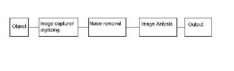
The acquisition of an image that is both focused and illuminated is one of the
most important parts of any machine vision system. Figure 1-2 shows the general steps
required in obtaining results from an image of an object.
Figure 1-2: Imaging flowchart
Originally the image capture and digitizing of the image was accomplished by using a
combination of a video camera and a frame grabber program (Russ, 2002). This method
has almost been entirely replaced with CCD (charge-coupled device) and CMOS
(complementary metal oxide semiconductor) chips. These chips use electrical circuits to
directly convert light intensities into a digital image. They combine the video camera and
frame grabber into one tool that can operate faster and with less distortion of the image.
These chips also have the advantage that they can produce images at a much higher
resolution then the frame grabber method (Russ, 2002).
Noise is the incorrect representation of a pixel inside an image. It is best observed in
variations in the color of a uniformly colored surface. Noise can be caused by numerous
electrical sources and its removal is important, since the noise can cause the features of
classified incorrectly. While many algorithms have been proven useful to remove noise,
the simplest method is to take multiple images of the same object and averaging the
images together (Russ, 2002). Since the noise is not the same in every image, when
averaged the noise will blend into its surroundings, making the resulting image much
clearer. Preprocessing of an image can include thresholding, cropping, gradient analysis,
and many more algorithms (Russ, 2002). All of the processes permanently change the
pixel values inside an image so that it can be analyzed by a computer. For example, in
grey scale thresholding, a value for the intensity is selected and any pixel whose intensity
value is less then the selected value intensity is set to 0 (black), if greater the value is set
to 255 (white). After thresholding, the resulting grey scale image can easily have features
classified and measured. The outputs from a machine vision system can be varied, in
robotics the output might represent the location of a object to be moved, in inspections
the output would be a pass or fall result, or in the case of this study the output is the
sweetpotatoes size and shape.
1.4.2 Classifying Mushrooms and Tomatoes using Machine Vision
A study by Nielsen and Paul showed that tomatoes can be more accurately
described by machine vision system than what is required by the USDA standards
(Neilsen et al, 1998). A study by Heinemann et. al (1994) used machine vision to grade
mushrooms. The system was trained from the results produced by one expert grader. The
which averaged 25%. The study concluded that misclassification was no worse for the
trained system than between the two expert graders (Heinemann et. al,1998). The study
showed that mushrooms can be described using a machine vision system. In summary,
these studies show the power that a machine vision system can have in classifying
agricultural products. Heinemann, et al. also showed that these systems are not perfect
and can still misclassify a product.
1.4.3 Classifying Apples and Potatoes using Machine Vision
Paulus, Busscher and Schrevens (1997) showed that a machine vision system
could be developed to describe an apple’s shape and color along with describing the
sources of human inconsistencies in grading; this was done by using a decision tree to
model human classification. Paulus and Screvens (1999) then expanded on this line of
research and looked into describing the shape of apple cultivars by using Fourier
expansion. Using principal component analysis, they indicated that the first two principal
components from the Fourier expansion is all that is needed to describe the overall shape
of an apple. The first principle component describes the height to width ratio and the
second principle component describes the conical profile of the apple. Then using the
developed Fourier expansion algorithms, the 12 “ideal” apple shapes as defined by the
“International Board for Plant Genetic Resources” were modeled in order to find their
fourier coefficients and principal components (Paulus et al, 1999). The ideal apples’
principal components were tested against six experimental cultivars and it was concluded
shapes. The second part of the study was to determine the number of profiles required to
accurately describe the apple. The conclusion was that four images at 90 degree intervals
can accurately describe an apples shape (Paulus et al, 1999).
Tao et. al (1995) investigated using machine vision on grading of potatoes on the
basis of shape. The shape of potatoes was determined by describing the boundary of the
profile using a radius fourier transform. Using the shape information, the algorithms
were tested and shown to obtain 89.2 percent correlation between human graders and the
computer. The ability to implement this system into a grading application is limited, since
the time required per root was shown be as high as two seconds.
In summary, these studies showed that the complex shapes of apples and potatoes
can be described using machine vision. The studies also showed that improvements
needed to be made in decreasing the inspection time in order to implement these
processes into a commercial grading procedure.
1.5 The use of Machine Vision with Sweetpotatoes
The work with classifying sweetpotatoes using machine vision has been limited,
with only two in depth studies being conducted. Both of the studies showed that the shape
of a sweetpotato could be classified in a quantitative manner using machine vision. The
first study by Wooten et. al (2000) looked into developing a yield and quality system that
would be used when harvesting sweetpotatoes. This study used a common machine
classified sweetpotatoes into four categories depending on their size and shape. In this
study shape was calculated using the polar moment of inertia. The study demonstrated
that based only on size the system would place the sweetpotato in the correct grade 80
percent of the time in the worse case scenario. When shape was included the success rate
would fall to 77 percent. The study also suggested that the system was more accurate if
the cull and jumbo sweetpotatoes were removed prior to inspection using the machine
vision algorithms (Wooten et al, 2000). The second study conducted by Wright, Tappan
and Sistler (1986) investigated the size and shape of sweetpotatoes. In the experiment a
sweetpotato was suspended in front of an imaging device and slowly rotated in order to
map its entire surface. The data was analyzed and it was suggested that the most logical
geometric shape match for a sweetpotato is a prolate spheroid and that a slight curve in
the major axis should be expected, based on the researchers expectations. Using the
equations for volume and surface area of a prolate spheroid the corresponding surface
area and volume were calculated. It was shown that the percent error in calculating both
surface area and volume of a sweetpotato when compared to the measured surface area
and volume was below six percent (Wright et al., 1986). This study indicated that the
prolate spheroid is a reasonable choice of a shape to represent the shape of a sweetpotato.
1.6 Objectives of this thesis
Consumers want produce to be of similar size and shape. They want the produce
to not only to look similar at the time of purchase, but from purchase to purchase at
has been left to human interpretation, based on a set of standards (CIP, 1981 and Jones et
al., 1969). Studies conducted for various agriculture crops, have demonstrated that using
machine vision can produce more accurate and uniform classification of the products
(Paules et al., 1997 and Heinemann et al., 1998). Several studies using machine vision
have been conducted on sweetpotatoes( Wooten et al,. 2000 and Wright et al,. 1986);
however none of these studies have produce a process to quantitatively measure the size
and shape of sweetpotatoes. Therefore, the goal of this project is to develop a machine
vision system that can accurately describe the visual physical characteristics of a
sweetpotato and create a numerical identifier that will contain all the characteristics in a
single sequence of numbers. The physical characteristics to be measured include the
sweetpotato’s width, length, length to width ratio and straightness. The description of
these characteristics inside a single number will allow for easier reporting of the
sweetpotatoes appearance instead of five individual numbers. This system will give
researchers a quantitative way a measuring the physical attributes of sweetpotatoes in a
way not available before. In order to accomplish this study the work was broken down
into three parts.
1. A hardware platform was developed to rotate the roots in a uniform
manner. The findings of Paulus et al, 1999, Wright et al., 1986 and
Wooten et al, 2000 were used as a guide in developing the system.
2. The use of an imaging device and lighting scheme was developed in order
obtain the best possible image.
2. Materials and Methods
This section discusses all of the components that were developed in order to
achieve the goals stated in the introduction. This section covers the design of the
hardware platform; the selection of the viewing device, and the development of all of the
algorithms used to measure the physical characteristics.
2.1 Hardware
A steady base was designed to provide a location that a viewing platform could be
attached as well as a location for the imaging device and lighting. The base was
constructed of 1.5 inch aluminum square tubing and 1.5 inch aluminum angle. The base
was built 42 inches high. The 1.5 inch angle was placed 7.5 inches down from the top and
12 inches up from the bottom. The aluminum angle lengths were cut so that the
rectangular base would have an outside diameter of 23.875 X 27.375. When assembled
the aluminum angle was positioned so that there was a flat base that viewing platform
could be mounted onto. Last, ½ inch plywood was mounted around the base in order to
block out the majority of the light and provide a location to mount lights and the imaging
device to. The plywood was mounted flush with the bottom of the 1.5 inch angle and to a
height of 18 inches above the top of the base. The base was made rectangular to provide a
long dimension that would provide enough distance to obtain the correct field of view
and a short dimension to allow for easy placement of sweetpotatoes onto the viewing
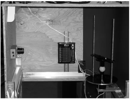
platform. Figure 2-1 shows the completed base, along with the position of the viewing
Figure 2-1: Picture of Completed Base
2.1.1 Viewing Platform
The viewing platform was responsible for holding the sweetpotato roots in
the correct orientation and to slowly rotate at a constant angular velocity. The rotation of
the roots is necessary, since Paulus et al (1999) showed that at least four views are
required to accurately describe the shape of an apple. Since both apples and
sweetpotatoes have irregular shapes, it was reasonable to assume that at least four views
the straightness of the sweetpotato, it was important that the angle the root has been
rotated can be accurately measured for each root.
The orientation of the sweetpotatoes inside the system was setup so that a line
drawn through the two ends of the sweetpotato would be parallel to the x-axis in the
produced images. The orientation of the sweetpotatoes is illustrated in Figure 2-2. The
z-axis comes straight out of the image and the grey dots represent the locations of edge
points found by the imaging device.
Figure 2-2 Orientation of the system
The original design had two power rollers positioned next to each other so the
sweetpotatoes would constantly rotate during the inspection process. A potentiometer
was attached to the power supply to control the speed at which the rollers would rotate. It
was originally assumed that the sweetpotatoes would become positioned and rotate, at the
same velocity of the rollers, and these rollers would provide the steady base. Several
trials were run with sweetpotatoes on this setup and it was found that angle the
sweetpotato roots, which caused sweetpotatoes of different shapes to rotate at different
rates.
To solve this problem, it was decided that a stepper motor with an attached
platform would provide the constant rotation necessary to make the required
measurements. The ability of the stepper motor to turn a set number of degrees provided
an extra benefit, in that the motion could be stopped after the required rotation had been
achieved. This allowed the imaging device to capture an image of a still object instead of
a rotating object, which provided an image that was less blurry.
An Applied Motion unipolar 5V with 200 steps per revolution was used in the
system. This stepper motor provided an angular resolution of 1.8 degrees per step. The
first attempt at controlling the stepper motor was to use a computer’s parallel port to
trigger a circuit that would rotate the stepper. Due to the low amount of power that a
parallel port can source, this approach was unable to consistently operate a circuit that
would operate the stepper motor. It was then decided that the IO ports from the imaging
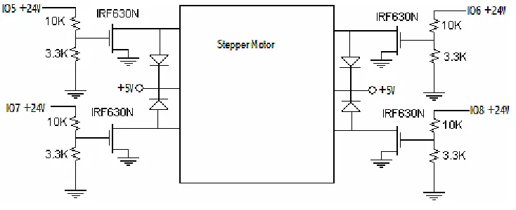
device could be used to control the motor. The following circuit, (figure 2-3), was
Figure 2-3: Stepper Motor Control Circuit
This circuit works by setting in sequential order the corresponding IO line, “high”, while
setting the other IO ports low. Using the equation for a voltage divider as shown below,
the resister values was chosen so that the voltage supplied to the MOSFETs
(Metal-Oxide-Semiconductor Field Effect Transistors)equaled 6 volts.
1 2 1
2
2 V
R R
R V
+
= ………..……. (1)
V2= output voltage
V1= input voltage = 24 volts R2= 3.3 KΩ
R1= 10 KΩ
The reduction from 24 volts to six volts was necessary to insure there was no damage to
the power MOSFETS. When the six volts are applied to the gate of the MOSFET, it
allows the current to flow through the corresponding coil of the stepper motor. When the
IO lines are run in succession, the stepper motor will rotate 1.8 degrees every time an IO
line is set high. The maximum speed at which the stepper motor can turn without a load
attached is determined by the turn-off time of the MOSFETS, which is 27 nanoseconds.
Once the stepper motor was operating a viewing platform that would be placed on
hold the sweetpotatoes in the correct orientation, during the entire inspection process. The
first viewing platform that was designed and built consisted of an 8 inch aluminum disk
with three slots cut 120 degree apart. Each slot is 3 inches long and a quarter inch wide.
The slots provided a location that three pegs can be positioned. Properly positioned, these
pegs held the sweetpotatoes upright and in the center of the disk. A hole was bored in the
center of the disk and a collar was inserted into the hole which allowed the platform to be
secured to the shaft of the stepper motor. The disk was made from aluminum to help keep
the weight of the platform at a minimum. This helped to ensure that the disk’s rotational
inertia would not exceed the holding torque of the motor, which would cause the motor to
skip a position and lose track of the angle the sweetpotato had been rotated. With the
addition of the platform the maximum speed at which the motor could operate was
reduced. Additionally, the maximum speed at which to motor could now be operated was
reduced since at high speed the sweetpotatoes often fell off the platform. This disk was
modified into a mandrel, when it was realized that is was difficult to ensure that the
sweetpotatoes were positioned correctly, so that the two tips produced a line that was
parallel to the y-axis in the images, during the entire inspection process. The mandrel
worked by using collars, with an inside diameter of 1/2”, to hold the ends of the
sweetpotatoes in the correct position. The bottom collar was attached to the original plate
by using the three slots. The top collar was attached to a bar that could have it’s height
above the plate adjusted and then secured by a thumb screw. The bar was allowed to slide
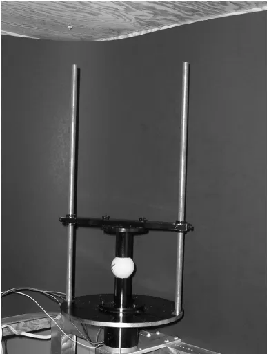
on two 16 inch long 0.375” round rods, that were screwed into the plated. By using the
entire inspection process. Figure 2-4, below, is an image of the completed viewing
platform.
2.1.2 Imaging Device
The imaging device that was selected for this project was a DVT 542c
Smartimage sensor (DVT). The 542c contains a 1/4” color CCD (charged-coupled
device) chip, with a 640 by 480 pixel resolution and contains a ring of 24 integrated
white LEDs to provide illumination. All DVT Smartimage sensors have a CS lens mount;
are powered by a 24V power supply and have both TCP/IP and serial communications.
DVT provides its own operating software, Framework, to control all its sensors.
Framework provides numerous preprogrammed image analysis algorithms and the ability
for additional algorithms, called scripts, to be developed and implemented on the 542c
using C++. Since the main purpose of any DVT system, is to be used in industrial
inspection, all of the preprogrammed DVT algorithms have been design for speed and
efficiency. This allows for quicker implementation since algorithms to remove noise,
detect edges and many more common machine vision processes do not need to be written
and optimized.
Using equation 2, a lens was selected to be used on the 542c. Knowing that the
542c has a CCD size of ¼”, the FOV needed to be 15” and the working distance could be
estimated at 20”. The focal length was determined to be 4mm.
WD FOV FL
CCD =
………. (2)
A Tamron CS mount 3-8mm zoom lens was selected for the system. The adjustable focal
length provides for adjustments in obtaining the proper focus for the system. Since the
lens is a CS mount it could be attached to the 542c Smartimage sensor without any
additional spacers. Figure 2-5, shows the 542c Smartimage sensor and lens attached to
the plywood base. The black wire on the left provides the 24V supply and serial
communications. The white wire provides the TCP/IP communications. The 542c was
position in the center of one of the plywood sides facing the opposite 23.875 side. The
Smartimage sensor was placed so that the CCD chip was positioned so that the resulting
images are oriented in such a fashion that the y-axis will run parallel to the minor axis of
the sweetpotato and the x-axis will run parallel to the major axis.
Figure 2-5: 542c Smartimage Sensor and Tamron lens
To provide lighting, two 18” fluorescent tubes were used. The fluorescent tubes,
tubes were determined by experimentation so that the position of the lights provides an
image that is both well illuminated and free from shadows.
2.2 Software
Once the hardware had been designed and built, software was written to control
the system and describe the physical characteristics of the sweetpotato. On power up, the
entire system is initialized. This initialization step powers up the camera and rotates the
stepper motor 4 steps. Since it is possible to rotate the platform freely when the power is
not connected to the motor, it is possible that the motor could be in aligned with any of
the four possible steps. Cycling through the four steps initially ensures that the motor will
rotate immediately when the inspection program is run.
The inspection program uses both Labview and DVT’s Framework to inspect and
determine the physical characteristics of the sweetpotato root. The Labview program is
Figure 2-6: Front Panel from Labview Program
The interface allowes the user to input the IP address of the 542c Smartimage sensor. It
also allows the user to control when an inspection is started along with ending the
inspections, which will close all communications between Labview and the 542c
Smartimage sensor. A green led was placed in the lower right corner to allow the user to
see when the program is inspecting. All the measured physical characteristics along with
the numerical identifier are displayed in the upper right hand side.
Once the start inspection button is pressed, the program enters the inspection
algorithm, shown in Figure 2-7. The 542c Smartimage sensor is programmed to run the
inspections of the root and will be explained in detailed in section 2.2.2.
{---}
If start inspection // waits until the start inspection button is pressed {
for image=0 to 6 // cycle through required images {
Inspect root // runs the algorithms for all characteristics Rotate stepper motor 36 degrees // turn stepper motor for next inspection If image=6 -- report characteristics and numerical identifier
Else – report busy // allows user to monitor progress of system }
}
{---}
The 6 images at 36 degree intervals were chosen because that number provides the
smallest number of images above four that had a uniform number of degrees between
images that could be obtained using this stepper motor. Four images at 90 degee intervals
were shown by Paulus et al, 1999 as the minimum number of profiles needed to describe
the shape of an object. A 36 degree interval was chosen based on the 1.8 degrees per step
resolution of the stepper motor. 36 degrees is achieved by stepping through each of the
four steps, five times. Once the inspection is completed the results are shown both on the
front panel of Labview and saved inside a user defined document. This inspection
program controls both the stepper motor and the inspection of the roots, whose
algorithms will be describe in the next two sections.
2.2.1 Stepper Motor Control
The control of the stepper motor was achieved by a combination of Labview and a
DVT background script. When the inspection algorithm is triggered by the start
inspection button, the string “trigger” followed by an end on line character is sent to the
DVT background script from Labview. The string is sent via a TCP protocol that is setup
between port 5005 of the computer and the 542c Smartimage sensor. The background
script, then triggers the inspection of the root. When the inspection is completed, IO lines
5-8 turned on and off in order five times. IO line eight is left on after the 5th cycle to both
stop the motion of the disk which allows for a cleaner image to be taken and to hold the
triggering the IO lines. During the entire inspection process the string is sent from
Labview to the background script a total of 6 times, once for each image.
2.2.2 Physical Characteristics
A total of four physical characteristics were measured in this study. These
characteristics are the sweetpotato’s width, length, length to width ratio and straightness.
Each of these characteristics contains their own unique algorithms to compute its
characteristic. Each characteristic is converted from number of pixels to millimeters of
length by multiplying the characteristic by a scale factor. The scale factor of .61
represents the physical size in millimeters that one pixel represents in the image. After
the sixth image is taken and inspected, all of the physical characteristics are computed
and sent to Labview via a TCP protocol set up between port 3247 on the computer and
the 542c Smartimage sensor. Labview takes this raw data and converts it into the
numerical identifier. The physical characteristics along with the numerical identifier are
then reported in the front panel of LabView, (Figure 2-6). All of the DVT script
algorithms are Labview program are located in Appendix B.
2.2.2.1 Width
Width has traditionally been one of the characteristics that could be measured
without the aide of machine vision system. A pair of calipers for example, is all that is
calculated by directly using a predefined DVT Softsensor. This characteristic is measured
using the Measure Across the Area Softsensor. A rectangular area inside the image was
setup from x equal to 9 to 200 and y equal to 39 to56. These numbers represent the x and
y pixel locations inside the image. Figure 2-8, illustrates the width algorithm. The
Softsensor is then set so that there is a scan line running parallel to the y-axis every other
pixel in the x direction. The scan lines work by scanning from the outside of the box to
the center of the box. The scan lines are set up to record the y position when a pixel’s
intensity goes above a threshold value; with each scan line reporting two edge locations,
an upper location and a lower location. Since the sweetpotatoes being measured are
smaller than the area being scanned, any scan lines that do not report an edge pixel are
Figure 2-8: Illustration of Width Algorithm
The light grey pixels that surround the sweetpotato represent the location of the
edge pixels. The edge pixels were found by setting the cutoff value for scan lines at 22
and conducting an open and close algorithm supplied by DVT. The open algorithm is a
machine vision process that erodes the object by set number of pixels, set at ten for this
system, and then dilates the object by the same number of image. The close algorithm
works in the same way expect it dilates and then erodes the object. When used in
conjunction these two algorithms help to eliminate any stray edge pixels that might have
be found on the mandrel used to hold the roots. The distance between the two edge points
on each scan line is calculated by the Softsensor. The maximum distance was then
reported as the width for each image. The largest width found from any of six images is
reported as the sweetpotato’s width in the raw data, which is sent to labview. This
process is the same as taking a caliper measurement every two pixels across the entire
length of the sweetpotato and recording the largest value obtained.
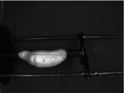
2.2.2.2 Length
Length is another characteristic that can be measured accurately without the aide
of machine vision. For this study, length was measured using the data collected from the
width algorithm. Using a DVT script Softsensor, length was defined as the x distance
between the first and last significant scan line. A significant scan line is any scan line that
length. The length that is being reported is shorter then the true length of the sweetpotato.
This is a result from the ends of the sweetpotato are hidden for view inside the two
collars used to hold the sweetpotato. However, it was assumed that ends that were being
hidden from view would not be of much use commercially, since they would have a
diameter smaller then 1/2'’ (12.7 mm). And the length that was being reported by the
system was a better representation of the sweetpotato’s length than just measuring tip to
tip. Figure 2-9, illustrates the output from the length algorithm. The grey line the runs
through the sweetpotato, illustrates the length that was measured by the length algorithm.
2.2.2.4 Length per Width Ratio
This characteristic is the only characteristic not computed using the 542c
Smartimage sensor. The length to width ratio is determined by dividing the reported
length from the Smartimage sensor by the reported width inside the Labview program.
This is important characteristic, since it provides a good gauge on the elongation of the
root. A small ratio would indicated that the sweetpotato is round, while a large ratio
would indicate a long narrow sweetpotato.
2.2.2.5 Straightness
The final characteristic this study will describe is straightness. Straightness is
defined as how straight the sweetpotato is along its long axis. This important feature,
which cannot be measured accurately or as fast by hand, has typically been included in
the shape classifications determined by CIP 1981, Jones et al., 1969, and Martin et al, 1983. The value of the straightness factor should equal zero when the sweetpotato is
perfectly straight and it should increase as the sweetpotato shape becomes more curved.
The expected number for the straightness of an ideal root should be somewhat above
zero, since Wright et al, 1986 showed that a slight curve in a sweetpotato’s shape should
The straightness is computed by using the scan lines used in the width Softsensor
to break the sweetpotato up into uniform sections that have a diameter equal to the
distance between the edge points and a width of 1.5 pixels. The center of mass for each
section is then used to compute the straightness factor. The next step in the straightness
algorithm is to compute the y and z coordinates of the center of mass for each section.
The x-coordinates of the center of mass for each section represent the significant scanline
that produced that section. Equation five was used to calculate the y and z coordinates of
the center of mass.
N t
t =
∑
' ………..… (5)Where: t is the coordinate of the center of mass being calculated t′ is the coordinate of the edge point
N is the total number of edge points
In computing the centers of mass for each section, the first step is to move the origin so
that the x-axis runs through a center of the sweetpotato root. The center of the
sweetpotato, yc′, is determined by averaging the two y′ values, of the edge points, in the
first scan line. The y′ stands for the y value measured by the 542c Smartimage sensor.
The first scan line was arbitrarily selected since the sweetpotato is placed on the viewing
platform vertical making the center axis of the viewing platform orthogonal to the middle
of the root. After yc′ is computed, two radii are computed from yc′ to the y′ position of
the two edge points for each section. These two radii represent the y′ distance from the
edge point discovered by the width algorithm can be computed. Equations six and seven
are the equations used to compute the y and z values for each scan line.
) cos( )
cos(
* θ lower θ
upper radius
radius
y= + ………. (6)
) sin( )
sin(
* θ lower θ
upper radius
radius
z= + ……….. (7)
Where: θ equals the angle the root has been rotated.
Radiusupper= y′ distance from center to upper edge point Radiuslower= y′ distance from center to lower edge point
The new x,y,z coordinate system were setup to match the coordinate system reported by
the 542c Smartimage sensor to avoid confusion. The y direction wass set to travel
vertically through the image and the z direction is then setup to come out of the image at
orthogonal to both the x and y axis, as illustrated in figure 2-11. Equation 6 and 7 sum
the two radii on each scan line for that image. After all y and z values have been
computed for every section in the image. The process of computing the y and z values is
repeated for each of the 5 remaining images. The y and z values from all six image are
then summed together from each section. The resulting sums result in the numerator of
equation 5 for both the y and z directions. Since six images are being summed together
the total number of edge points for each section equals 12. Using this information and
equation 5 the y and z coordinates for the centers of mass for each section can then be
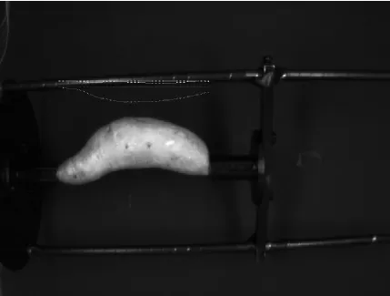
determined. The locations of computed the centers of mass for the straightness algorithm
is illustrated in Figure 2-10. The top curved line represents the location of the z center of
mass. The top straight line represents the location of the z center of mass if the
sweetpotato has no bend. The bottom curved lines illustrates the positions of the y centers
of mass. The bottom straight line represents where the y center of mass would be if there
Figure 2-10: Illustration of Computed Centers of Mass
Using the centers of mass computed by the routine above the straightness factor
can now be calculated. Starting with the second significant scan line, the differences
between the coordinates of the center of mass between the current scan line and the one
prior are calculated and then squared. Since only the amount of bend is being investigated
the squaring the results allow for negative values to be eliminated. The squaring also
protects against the case of a “S” shaped sweetpotato, whose straightness would be
reported as zero since it would have equal positive and negative differences. Only the y
being added together, until the difference between last significant scan line and its
predecessor is calculated. The total change in both the y and z directions is then added
together. This resulting sum has its square root calculated to nullify the squares being
calculated previously and is reported as the straightness factor. The square root was
calculated to help reduce the size of the number caused by squaring all of the numbers.
2.2.3 Numerical Identifier
The numerical identifier is used to combine the results from all the physical
characteristics into one 15 digit code. Since the numerical identifier contains six physical
characteristics that have been measured quantitatively, the numerical identifier will be a
more accurate way of describing sweetpotatoes than the processes described by CIP 1981,
Jones et al., 1969, and Martin et al, 1983. This numerical identifier is produced by a
combination of two DVT scripts and Labview. The first DVT script receives data from
the width, length and effective length factors after each image is analyzed. This script
compares the results from each image and reports the largest length and width found. The
second background script reports the straightness and shape factors it receives after the
sixth image is analyzed. These two scripts are combined into a single string of data that
contains all the characteristics, with each characteristic separated by a comma. This string
is then sent via a DVT application call Datalink to Labview. Datalink sets up the TCP
protocol between Labview and the 542c Smartimage sensor. As Labview receives the
data it breaks the string apart into the characteristics. Wooten et al in 2000 reported that
justifiable to believe that both the shape and straightness factor computed would behave
in a similar fashion. To solve this problem the straightness number was normalized by
dividing both characteristics by the sweetpotato’s length. This results in straightness to
be reported on a per millimeter of length basis and allows for comparison straightness
between roots that are not of the same size. The modification of straightness is
acceptable, since only the magnitude is needed for the comparison to other sweetpotatoes,
is needed. All of the results are converted into an integer value to get rid of the decimal
places, except for straightness which remains a floating point number with three numbers
following the decimal place. The new results for length to width ratio and straightness are
then combines in Labveiw into the 10 digit numerical identifier, illustrated in Figure
2-11.
W W L L L R ST . ST ST ST
W- Width R= Ratio of Length to Width
L= Length ST= Straightness
3. Results and Discussion
This section provides the results from the inspections of five standard shaped
objects and ten sweetpotato roots. The five standard objects include three round spheres
of diameters of 37, 62, and 65 mm respectively and two different sized mini footballs.
The sweetpotato roots were purchased on the same day at a local supermarket. Each
object was inspected 30 times to produce a set of thirty numerical identifiers. The results
were then averaged to produce the arithmetic average measured value for each
characteristic. These results were analyzed to illustrate the effectiveness of the developed
system and algorithms.
3.1 Standard Objects
The five standard shaped objects were selected to illustrate the ability of the
system to produce accurate results. The three spheres, with a sphere being a prolate
spheroid with equal major and minor axis, were chosen to demonstrate that the system
would produce a straightness factor equal to zero. The footballs were chosen since they
have a shape that is similar to a sweetpotato and have a straight major axis. The following
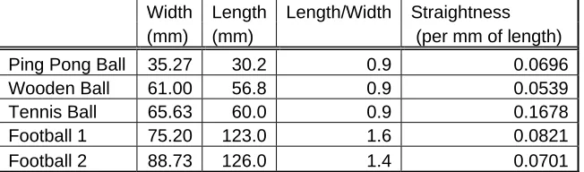
chart (Table 3-1) illustrates the arithmetic average of the characteristics for the standard
Width Length Length/Width Straightness (mm) (mm) (per mm of length) Ping Pong Ball 35.27 30.2 0.9 0.0696 Wooden Ball 61.00 56.8 0.9 0.0539 Tennis Ball 65.63 60.0 0.9 0.1678 Football 1 75.20 123.0 1.6 0.0821 Football 2 88.73 126.0 1.4 0.0701
Table 3-1: Results of Five standard objects
All three spheres and the two footballs had their widths measured within two
millimeters of their actual diameters. This small amount of error is the result of the
method of finding the edge pixels inside the width algorithm. The width algorithm was
set up to detect an edge pixel when the normalized intensity reached 20. This results on
edge pixels being placed on the inside of the edge, instead of the outside. Doing this,
resulted in the widths being reported 2 pixels or 1.22 millimeters small. The algorithm
could have been set up to report the edge pixels on the outside of the edge; however this
would have resulted in the widths being 1.22 millimeters to large. The rest of the two
millimeters of error is the result of the placement of the scan lines at every other x value.
This could result scan line not running along the true maximum width; thus reporting a
width slightly smaller the actual width is possible. The lengths for the three spheres were
reported to be approximately five millimeters smaller then the widths. This was expected
since the length algorithm was developed to report the length from that the object has a
diameter greater then 1/2”. The lengths reported for the footballs were both
approximately ten millimeters smaller then the measured lengths. This larger difference
measured. The straightness factors for the ping-pong ball, wooden ball and tennis ball
was measured at 0.0696, 0.0539, and 0.1678 respectfully. The small difference from zero,
for the ping pong ball and the wooden ball is the result of rounding during the
computation of the straightness factor. The large value for the tennis ball can be
attributed to the black lettering on the ball. This lettering only occurs on one side of the
ball could, on some views, cause an incorrect reporting of the edge pixels. These
incorrect edge pixels would then cause the centroids to be calculated incorrectly. The two
footballs also small straightness factors of 0.0821and 0.0701 respectively. These results
were slightly larger then the straightness numbers for the ping pong ball and the wooden
ball. This small difference is believed to be caused by the plastic laces on the footballs
showing up in a view.
Overall the results from the standard objects showed that the system would
measure all of the physical characteristics and produce results that were reasonable. The
width for all of the standard objects measured by the system agreed within 2mm of the
width measured by hand. The measured lengths were smaller then the lengths measured
by hand. This was expected, since the length was set up to measure a length shorter then
the actual length. The straightness numbers produced by the system agreed with what was
expected. The tennis ball showed that discoloration can cause results for shape and
straight to diverge from what is expected, by producing incorrect locations for edge
pixels.
It is important to comment on how uniform the results for the physical
characteristics were. Table 3-2, below, provides the standard deviations for each of the
Width Length Length/Width Straightness Ping Pong Ball 0.450 0.551 0.017 0.018
Wooden Ball 0.000 0.551 0.009 0.005 Tennis Ball 0.490 0.000 0.007 0.012 Football 1 0.407 0.000 0.009 0.006 Football 2 0.583 0.000 0.009 0.004
Table 3-2 Standard Deviations for the Standard Objects
For all of the objects the largest standard deviation for the width or length was
0.583 millimeters. The uniformity of the results suggested that the system will produce an
accurate measurement of symmetrical object every time it is inspected, regardless of its
initial position in the system. If the standard deviations have had been larger, it would
have suggested that position of the object or the viewing platform had some affect on the
measurement of the characteristics. The standard deviations for straightness was largest
for the ping pong ball, this is believed to be the result of the small size of the ping pong
ball. The tennis ball also had a large standard deviation when compared to the wooden
ball or either of the footballs. The large standard deviation was due to the black lettering
on the tennis ball. The reasoning that the lettering could cause the larger standard
deviations was its different locations in different inspections, in some inspections the
lettering fell on the edge of the profile causing larger error while during others it did not.
The variation in the results footballs and the wooden ball are believed to be mainly
caused by rounding errors, however part of the variation in the results is believed to be
caused by the mandrel used to hold the objects blocking part of the profile. To get a better
characteristics were normalized by two different methods. The normalization allows for
the comparison of the deviations of objects of different sizes, to see if there was any
possible correlation between the deviations. The first method for normalization was
conducted by dividing the standard deviation by the measured length of the object. The
second method for normalization divided the standard deviation of the characteristic by
characteristic’s measured value. The normalized data was placed in Tables 3-3 and 3-4.
Since the objects being inspected are symmetrical objects, each of their six profile images
should be the same regardless of the objects initial orientation. Any variation in the
profiles captured by the 542c SmartImage sensor would be caused by the mandrel used to
hold the objects, obstructing the view of the 542c. The mandrel had been painted black to
help them blend into the background. However it was still possible that it could cause
variations in the results. For the system to be functioning correctly, it is important to
show that the system was not causing any uniform error that could be adjusted adding a
correction factor to any of the characteristics. Correction factors could easily have been
included in any of the algorithms to nullify any effects the system might have on an
Normalized by Length
Width Length Length/Width Straightness Ping Pong Ball 0.0149 0.0182 0.0006 0.0006
Wooden Ball 0.0000 0.5916 0.1674 0.0001 Tennis Ball 0.0082 0.0000 0.0409 0.0001 Football 1 0.0033 0.0000 0.1069 0.0001 Football 2 0.0046 0.0000 0.1350 0.0001
Table 3-3: Standard Deviations Normalized by the Object’s Length
Normalized by Characteristic
Width Length Length/Width Straightness Ping Pong Ball 0.013 0.018 0.020 0.264
Wooden Ball 0.000 0.010 0.010 0.095 Tennis Ball 0.007 0.000 0.007 0.073 Football 1 0.005 0.000 0.005 0.075 Football 2 0.007 0.000 0.007 0.053
Table 3-4: Standard Deviations Normalized by the Characteristic
In both methods of normalization; the normalized standard deviations do not appear to
have any pattern that would indicate any common error that is being caused by the
system. This would suggest that the variations in the results are from computing the
measurement or rounding the results into integers and not the mandrel used to hold the
objects. This would suggest that the mandrel not causing any error in the calculations and
a correction factor for any of the characteristics is not needed. The only object that
appears to be affected by the system was the ping pong ball, which had a normalized
standard deviation significantly larger then the others. Since, the ping pong ball is of such
small size, it is logical to conclude that the any common error between to objects would
appear to be magnified in an object that small. This error should not be a problem in the
of these characteristics. However a correction factor of 1.22 millimeters will be added to
width to correct for the under measurement of the width caused by method edge pixels
are located.
Overall the system was shown to produce measurements for the width, length,
ratio of length to width and straightness for all of the standard objects that are
independent of the position of the mandrel or their orientation in the system. The system
produced straightness factors that matched what was expected, with all the objects having
very small straightness numbers. The lettering on the tennis ball showed that a black
discoloration on an object could cause the system to misplace edge points, resulting in
incorrect measurements for straightness.
3.2 Sweetpotatoes
After the system had been shown to measure several standard objects, ten
sweetpotatoes were inspected to show that the system could measure all of the physical
characteristics of sweetpotatoes. The results from the inspections will also be used to
illustrate the amount of variation in the size and shape of sweetpotatoes that can be found
at a local supermarket. The results from the two mini footballs will be included in the
data to provide a comparison of a sweetpotato to an object with approximately the same
profile.
As with the standard shapes, all ten sweetpotatoes were inspected 30 times. The
results for each characteristic were then averaged together to produce an arithmetic
illustrated in Figure 3-1 and the results from shape and straightness illustrated in Figure 3-3. 0 25 50 75 100 125 150 175 200 225 250 Sweet potat o 1 Swee tpotat o 2 Sweet potat o 3 Sweet potat o 4 Sweet potato 5 Sweet potat o 6 Swee tpotat o 7 Sweet potato 8 Sweet potat o 9 Sweet potato 10 Footba ll 1
Foot ball 2
Rat
io x10, S
tr a ig htn ess x10 3 Width (mm) Length (mm) Ratio
Straightness (per mm or length)
Figure 3-1: Results for Width, Length, Ratio, and Straightness of Sweetpotatoes and Mini Footballs
The system measured the average widths of the ten sweetpotatoes as 43.6, 69,
57.6, 57.5, 53.1 53.8, 51, 47.1, 44, and 53 millimeters. Using the data from all 30
inspections, 95 percent confidence intervals for each of the sweetpotatoes width were
constructed, shown as the plus/minus bars on Figure 3-1. The produced confidence
intervals did not contain any of the widths measured by hand of 45, 67, 59, 55, 54, 55, 49,
42, 48, and 56 millimeters, respectively. Since the 95% confidence intervals were of
system can measure the correct value for width and just how difficult it is to measure the
size of a sweetpotato. The lengths that were measured produced results with small 95%
confidence intervals. Knowing that standard objects had their lengths measured correctly
and the sweetpotatoes had small confidence intervals in the results; the data suggests that
the system is measuring the correct lengths. These results demonstrated that the system
can measure that width, length, and ratio of length to width of sweetpotatoes. The
uniformity of the results as illustrated by small standard deviations, suggests that the
same results for a sweetpotato will be obtained regardless of the original position of the
sweetpotato in the system.
The straightness numbers were larger for the majority of the sweetpotatoes than
the straightness numbers for the footballs. This appears to help to validate the findings of
Wright et al. (1986) that showed a slight bend in the major axis of the sweetpotato. The
confidence intervals for straightness were considerably larger than the confidence
intervals for the other characteristics. The larger confidence interval is believed to be
caused by only using six images. By only using six images and given the sweetpotato’s
naturally irregular shape, it is possible to not capture the same six profiles each time an
inspection is run. The variation in these profiles would create varying straightness
numbers and result in the larger confidence intervals. This is best illustrated by the range
in the straightness confidence intervals for the footballs compared to the sweetpotatoes.
The footballs, which have a uniform profile from any angle had smaller confidence
intervals than the intervals for the sweetpotatoes.
The straightness number was not a sensitive to the bending of the major axis as
Sweetpotato Three Sweetpotato Ten Figure 3-2 Illustration of Sweetpotato Three and Ten
Visual inspection of sweetpotato three and ten would suggest that sweetpotato
three should have a much larger straightness number. The results however in Figure 3-1
would seem to indicate that the curvature of sweetpotato three was not much larger then
sweetpotato ten, the 95% confidence intervals for sweetpotatoes three and ten. While the
straightness number did not increase as much as was expected, it did show an increase in
the result as the amount of bend increased. Overall the straightness factor did not have as
large of variation as was hoped, however it did show that the amount of bend could be
measured.
The observation that the system would measure the same characteristics,
regardless of initial position, was tested by reinspecting all ten sweetpotatoes. For this
test each sweetpotato was inverted from it’s original position and tested again. The
Width (mm) Length (mm) Ratio Straightness (per mm of Length)
Inverted Inverted Inverted Inverted p-value Sweetpotato 1 43.6 43.50 173.9 172.7 4 4 0.1067 0.1371 0.311
Sweetpotato 2 69.0 68.73 122.3 122.1 2 2 0.1243 0.1262 0.083 Sweetpotato 3 57.5 57.10 160.9 161.0 3 3 0.2094 0.2288 0.008 Sweetpotato 4 47.0 47.67 109.4 109.7 2 2 0.1128 0.1201 0.158 Sweetpotato 5 53.8 53.80 149.4 149.3 3 3 0.2224 0.2099 0.109 Sweetpotato 6 51.0 51.63 90.3 91.5 2 2 0.1453 0.1184 1.08E-05 Sweetpotato 7 53.3 53.30 120.7 120.6 2 2 0.2107 0.1960 0.001 Sweetpotato 8 47.1 47.23 143.5 143.0 3 3 0.1233 0.1294 0.052 Sweetpotato 9 44.0 44.00 143.5 143.6 3 3 0.1386 0.1448 0.031 Sweetpotato 10 53.1 52.80 185.2 185.0 3 3 0.1911 0.1896 0.656
Table 3-5: Results from Inverting Ten Sweetpotatoes
The largest variation between the average results of width and length were observed to be
approximately 0.67 millimeters for the width and 1.2 millimeters for the length. The
variations accounted for only approximately 1% of the total width or length and are
considered acceptable given the large variations in the size of sweetpotatoes allowed in
the US No. 1 grade for sweetpotatoes. This demonstrates that the position of the
sweetpotato has little effect on the measurement of its width or length. The results for the
straightness number appear to be similar. As a check to see if the results for straightness
were not significantly different, a paired two-sample student's t-test, with an alpha level
of 0.05 and hypothesized mean difference of zero, was conducted on the straightness
numbers. The p-values from this test showed that for sweetpotatoes three, six, seven and
nine had means that were significantly different. While statistically significant, the
variations were still inside the confidence intervals produce in Figure 3-1. This would
suggest that the variation is a result in only using six images to describe the sweetpotato’s
The results from the ten sweetpotatoes illustrate that the system will accurately
measure the length, width, effective length. By inverting the sweetpotatoes the system
demonstrated that these measurements can be made regardless of the sweetpotatoes
position. The system was demonstrated to have the ability to quantify the sweetpotatoes’
straightness. The quantification method straightness however, causes some slight
variation in the results, of multiple inspections of the same sweetpotato; depending on the
orientation of the system and the sweetpotato. This is believed to be primarily, the result
of only using six profiles to inspect the root. The main causes of error in the calculation
of length, width and ration of length to width are believed to be caused by rounding
errors in the calculations of the characteristics. The findings for straightness appeared to
confirm the findings of Wright et al. (1986) that a slight bend in the major axis of a
sweetpotato can be expected. The results for the sweetpotatoes show that the amount of
variation in shape of sweetpotatoes that are sold in grocery stores is highly variable. This
is the opposite of expectations of consumers, who typically desire produce to have similar
4. Conclusions
This study looked into the use of machine vision to produce numerical identifiers
that represent several physical characteristics of sweetpotato roots. The developed
system was tested using five standard objects and ten sweetpotatoes. The results
demonstrated that the developed algorithms could measure the physical characteristics.
The resulting system achieved all three objectives that were stated in the introduction.
1. The developed system provided a method for uniformly rotating the
sweetpotatoes. The rotation was achieved by a stepper motor that is controlled by
I/O ports on the DVT 542c SmartImage Sensor. The developed viewing platform
provided the stable and adjustable location needed to hold the sweetpotatoes in
the correct position for inspection. An aluminum frame covered by plywood was
constructed to block the majority of the outside light and provide a platform to
mount the hardware to.
2. A DVT 542c SmartImage sensor and a Tamron 3-8mm zoom lens were selected
to acquire the images of the sweetpoatoes. The selected lens provided the 15”
field of view needed to image all possible sweetpotato sizes. The 542c
SmaertImage sensor was placed in the center of the plywood side opposite of the
viewing platform. Two white 18” fluorescent lights were placed at 6” above and
one six inches below 542c. The location for the lights provided the best
illumination, with the least shadowing of the objects. The viewing platform and
the plywood side behind the sweetpotatoes were colored black to provide the best