L. De Angelis,1 F. Alpeggiani,1 A. Di Falco,2 and L. Kuipers1,∗
1Center for Nanophotonics, AMOLF, Science Park 104 1098 XG Amsterdam, The Netherlands 2
SUPA, School of Physics and Astronomy, University of St Andrews, North Haugh, St Andrews KY16 9SS, UK
(Dated: July 22, 2016)
Phase singularities are dislocations widely studied in optical fields as well as in other areas of physics. With experiment and theory we show that the vectorial nature of light affects the spatial distribution of phase singularities in random light fields. While in scalar random waves phase singularities exhibit spatial distributions reminiscent of particles in isotropic liquids, in vector fields their distribution for the different vector components becomes anisotropic due to the direct relation between propagation and field direction. By incorporating this relation in the theory for scalar fields by Berry and Dennis, we quantitatively describe our experiments.
PACS numbers: 05.45.-a, 42.25.-p, 02.40.Xx
Finding correlations in chaotic systems is the first step towards understanding. Many are the fields where such predictions could be exploited, from weather forecast to economic modeling [1, 2]. The study of random phe-nomena is a topic of great interest and inspiration for many branches of physics as well. In electromagnetism, for example, random wave fields have been a topic of intense studies since decades, an outstanding example being Anderson localization of light [3]. More recently the scientific interest on random wave fields has contin-ued intensively, ranging from useful techniques as non-invasive imaging with speckle correlation [4] to fascina-tion concerning the observafascina-tion of rogue waves in optical fields [5, 6]. Zooming into the structure of a random wave field, attention has been pointed to deep-subwavelength dislocations known as phase singularities [7].
Phase singularities are locations in which the phase of a scalar complex field is not defined. In two-dimensional fields these locations are points in the plane. Although they are just a discrete set of points, phase singularities can describe the basic properties of the field in which they arise. For this reason they are widely studied in wave fields [8–14], as well as in many areas of physics, where they are better-known as topological defects in ne-matics [15] or as vortices in superfluids [16].
For a single frequency phase singularities are fixed in space, and their spatial distribution in a scalar field of monochromatic random waves has been analytically modeled by Berry and Dennis [17]. The hallmark of such a distribution is a clear pair correlation, reminiscent of that of particles in liquids. By realizing random waves ensembles in microwave billiards [18–20], the correlation of phase singularities was tested for a field perpendicu-lar to the plane of the billiard, showing excellent agree-ment with the theoretical expectations [21]. For such a field and in that geometry indeed scalar theory was ap-propriate. However, electromagnetic waves are vectorial in nature, and in a different framework it was already demonstrated how the presence of a spin degree of free-dom can affect the correlation properties of a ranfree-dom
field [22, 23].
Here, we show how the vectorial nature of light affects the distribution of its phase singularities. By mapping the in-plane optical vector field measured above a chaotic resonator we investigate the distribution of phase sin-gularities in two-dimensional random vector waves. We show that the distribution of phase singularities devi-ates from that for scalar random waves. This deviation is caused by the relation between the transverse field and waves propagation direction. Thus, even when the considered vector field is equipartitioned with respect to both the in-plane polarization and propagation direction, any specific choice of field component directly leads to an anisotropic distribution of the contributing propagation directions. By treating this anisotropy with an analytical model we quantitatively explain our experimental obser-vations. Finally, we show how an out-of-plane component that we construct from our in-plane fields obeys the pre-dictions for scalar fields.
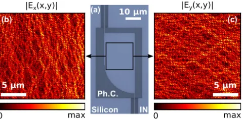
To generate optical random waves we inject monochro-matic light (λ0 = 1550 nm) in a chaotic cavity: a silicon-on-insulator membrane enclosed by a planar pho-tonic crystal with one input and one output waveguide [Fig. 1(a)]. Light is coupled through the input waveg-uide, exciting a Transverse Electric (TE) slab mode in the silicon membrane, which has its electric field vector in the membrane plane.
With our near-field microscope we map the in-plane components of the optical field in the cavity, which is in fact the only non-vanishing component of the electric field. The near field is locally converted and delivered to the far field through an optical fiber. A heterodyne detection scheme enables the measurement of amplitude and phase [24]. With standard polarization optics we selectively detect the (Ex, Ey) Cartesian components of the in-plane electric fieldE[25], thus gaining access to its vectorial content. By scanning the surface of the sample we measure a two-dimensional map of the in-plane com-plex optical field above the cavity.
FIG. 1. Near-field measurement of the amplitude of the two cartesian componentEx (b) andEy(c) of the optical electric
field in theChaotic Cavity (optical micrograph shown) (a).
ofEx andEy. The field pattern that results in the cav-ity can be thought of as a random superposition of plane waves [20]. We find that for the x- and y-components of the field the probability density function of the inten-sity is exponential [26], underlying the randomness. The near-field maps [Fig. 1(b),(c)] depict the patterns result-ing from interference of light in the chaotic cavity. At first sight destructive and constructive interference occurs at random locations in the plane. On closer inspection a difference between the maps of the two field components catches the eye: the features of each pattern exhibit a preferred axis, related to the specific field component. A vertical stripy pattern with roughly 1−2 micrometers between the stripes is present in theEx field. A modu-lation of the amplitude is observed along the stripes as well, characterized this time by a shorter length scale. The case ofEy is completely analogous, but rotated by 90 degrees.
By separately measuring the Cartesian components of the electric field we implicitly established a criterion to depict a vectorEby using two scalar quantities (Ex, Ey), in which we can now seek for phase singularities [27]. Please note that such singularities cannot be found in the total intensity, which has no vanishing points. In a two-dimensional scalar complex fieldψ(r), phase singularities are points in which its phase ϕis undefined. The phase circulates around the singular points, assuming all its possible values from−πtoπ[7]. Quantitatively, the line integral ofϕalong a pathCenclosing only one singularity yields an integer multiple of 2π:
Z
C
dϕ= 2πs, (1)
where the integersis calledtopological charge of the sin-gularity. The definition of topological charge also gives us a powerful way to identify phase singularities. We calculate the integral of Eq. (1) along 2×2 pixels loops at every point of the measured phase map, determining position and topological charge of all the optical vortices in the field, with a spatial accuracy that is limited by the pixel size, of approximately 20 nm. Figure 2 shows the
50 nm
Positive Singularities Negative Singularities
[image:2.612.58.298.51.170.2]0.5 μm -π 0 π
FIG. 2. False-color map of the measured phase ofEx. Phase
singularities are represented (circles) with their topological charge: +1 (positive) or -1 (negative). The zoom highlights how the direction of the circulation of the phase around the singular point determines its topological charge.
phase singularities pinpointed in a subset of the phase map ofEx. Only topological charges of±1 are observed. The distribution of optical vortices in the plane is rather disordered (Fig. 2), although already by eye a spa-tial correlation seems discernible if taking into account the topological charge. In order to to unveil such corre-lation we quantitatively characterize their spatial distri-bution. A natural way to do this is by calculating the pair correlation function
g(r) = 1
N ρh
X
i6=j
δ(r− |rj−ri|)i, (2)
where N is the total number of singularities, ρ is the average density of surrounding singularities and δ the Dirac function. This function is directly related to the probability of finding two entities (riandrj) at a distance
rfrom each other and is widely used in physics to describe discrete systems of various kinds [28].
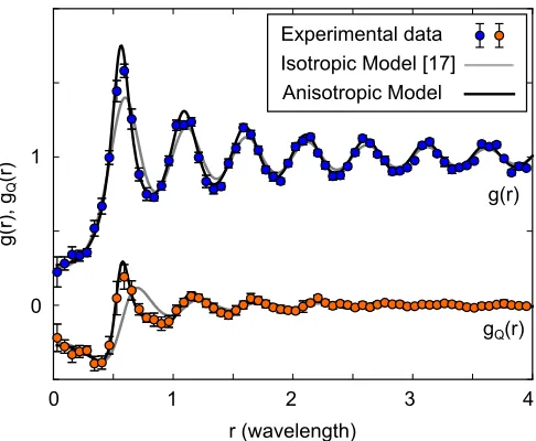
Figure 3 presents theg(r) calculated from our experi-mental data, specifically for the full data set of singular-ities ofEx [29]. The shape of the distribution function is highly similar to what is typically observed for a sys-tem of particles in a liquid [28]. After an initial dipg(r) oscillates around one, with an amplitude that decreases asris increased. The first peak, representative of a sur-plus of singularities, emerges at a distance of roughly half a wavelength. The decrease in amplitude of the os-cillations describes the loss of correlation of the system. However, one peculiarity that we observe is definitely dif-ferent compared to the case of a liquid: g(r) approaches a finite value forr≈0. This means that asymptotically there is a finite probability of finding two vortices at the same location. While unusual this is in fact allowed by the zero-dimensionality of optical vortices.
r (wavelength)
g(r)
, g
Q
(r)
g(r)
0 1
0 1 2 3 4
Experimental data Isotropic Model [17] Anisotropic Model
gQ(r)
FIG. 3. Pair (blue) and Charge (orange) correlation function of phase singularities in the measured fieldEx. The gray line
is the theoretical expectation for a scalar field of isotropic random waves [17]. Our data significantly deviates from such theory, while a perfect agreement is obtained by considering a new model that includes directional anisotropies (black lines).
it is convenient to introduce a generalized expression of the g(r) for a system of charged entities. In thecharge correlation function gQ(r) each vortex is weighted with its topological charges:
gQ(r) = 1
N ρh
X
i6=j
δ(r− |rj−ri|)sisji. (3)
The experimental result for the gQ(r) is also reported in Fig. 3, providing new information about our system. The main observation here is thatgQ(r) is approximately equal to−g(r) in the regionr≈0, meaning that only sin-gularities with opposite topological charge are likely to be indefinitely close to each other. This behavior is usually interpreted in terms of reciprocal screening among criti-cal points with opposite topologicriti-cal charge [30, 31]. No-tably, critical-point screening is related to the reduction of topological charge fluctuations inside a finite region with respect to the prediction for a collection of random charges [17, 30, 32].
In an influential paper [17] Berry and Dennis calcu-lated the correlation functions of singularities in a scalar field ψ, modeled as a superposition of plane waves with the same momentum and random phasesδk, i.e.,
ψ(r) =X k
akexp(ik·r+iδk). (4)
The model assumes that the waves amplitudes are isotropically distributed along a circle of radius k0 in Fourier space. The results of this isotropic model are shown as solid gray lines in Fig. 3. Most of the key fea-tures of the experimental distribution are qualitatively
accounted for by the model, but we clearly observe some deviation from the theory. The biggest difference is in thegQ(r), where the first peak turns out to be narrower than in theory, as well as significantly shifted towards lower distances. This is in contrast with what was ob-served for out-of-plane fields in microwaves billiards [21], where excellent agreement was found.
The origin of the observed discrepancies with respect to g(r) and gQ(r) lies in the vector nature of the light. For the TE modes a direct relation exists between the selected in-plane field component and the direction of propagation: the modes will have no electric field com-ponent along the direction of propagation. Therefore the choice of field component to be investigated (e.g. Ex in Fig. 2) affects the distribution of propagation directions that contribute to the wave pattern. Whereas the gen-eral model in Eq. (4) remains valid, the anisotropy of our system violates the assumption of isotropy [17], i.e., thatak only depends on the magnitude ofk. As a con-sequence, the field correlation function must display an additional dependence on the relative spatial orientation of the points.
We now calculate the correlation properties of the in-plane components of the field and of the corresponding singularities distribution, by including such anisotropy in a modified version of the original model. Since for a TE mode E(k)⊥k, the Fourier coefficients of the in-plane field components are effectively modulated by the sine of the angleθk enclosed by the direction of the considered field component and the in-plane wavevectork. For this reason, we assume
Ej(r)∝ X
k
sin(θk) exp(ik·r+iδk), j =x, y. (5)
Note that the total intensity,E2
x+Ey2 remains isotropic. The additional angular dependence in the Fourier ex-pansion of Eq. 5 influences the correlation properties of the wave field. In particular, the spatial autocorrelation function of each field component,
C(r) = Z
dr0Ej∗(r0)Ej(r0+r) = 1 2π
Z
dk|Ej(k)| 2
e−ik·r,
(6) exhibits a dependence on the orientationϕof vectorr:
C(r)=. C(r, ϕ) = 1 2π
Z
dθk sin2(θk)e−ik0rcos(θk−ϕ)(7)
= 1
2[J0(k0r) + cos(2ϕ)J2(k0r)], (8) where Jn(x) is the Bessel function of order n and k0 is the wavenumber of the TE mode. This is in con-trast with the case of a fully isotropic scalar field, where
[image:3.612.56.299.49.249.2]Anisotropic Model
0 1 2 3
0 1 2
r (wavelength)
Ex
0
gQ(r) gQ(r) Experimental Data
gQ
(
r
[image:4.612.64.292.49.239.2])
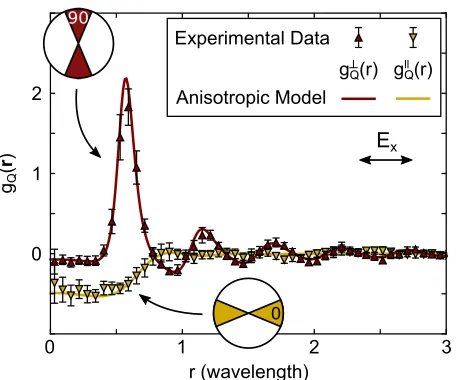
FIG. 4. Directional charge correlation function. We repoort the two illustrative cases of direction perpendicular (red) or parallel (yellow) to the direction of the considered field com-ponent (Ex). The distribution function strongly depends on
the direction in the plane. Experimental data is represented by the triangles, while lines show our modified model for anisotropic random waves, which perfectly fits the data.
correlation functions, g(an)(r, ϕ) and g(an)
Q (r, ϕ), display a dependence on the spatial vector orientation ϕ. Since in the corresponding experimental quantities in Eqs. (2) and (3) the average is taken over all reciprocal orienta-tions of the points, to compare the experimental data with the theoretical results, we average the latter over the polar angle:
gQ(an)(r) = 1 2π
Z 2π
0
dϕ gQ(an)(r, ϕ) (9)
[image:4.612.318.563.456.652.2][and similarly for g(an)(r)]. The black solid lines in Fig. 3 show the analytic outcome of such calculations (Anisotropic Model). Comparison between experiment and the new model now exhibits an excellent qualita-tive and quantitaqualita-tive agreement. This confirms that the anisotropy in the direction distribution of random waves, intrinsic in the vector nature of optical wave fields, sig-nificantly affects the spatial distribution of phase singu-larities.
A further confirmation of the validity of our model comes from restricting the orientation of the spatial dis-placement vector r to a limited range of values (∆ϕ =
π/4) around the directions perpendicular (⊥) and par-allel (k) to the field projection axis. In Fig. 4, we com-pare the results for both the experimentally calculated
gQ(r) and the restricted averages of Eq. (9) (Anisotropic Model). The two direction-dependent distribution func-tions show a completely different behavior, neither being equal to the isotropicgQ(r) of Ref. [17], which, of course, does not display any orientation dependence. Several dif-ferences can be spotted betweengkQandg⊥Q. First,gQ⊥(r)
vanishes asrapproaches zero, whilegQk(r) does not. As a consequence singularities of opposite sign are most likely to be arbitrarily close along the polarization direction. Secondly, in theg⊥Q(r) there is an evident and positive peak, followed a number of clear peaks with decreasing height. Sequences of same-sign singularities spaced by approximately half a wavelength are therefore expected along the direction perpendicular to the polarization (see also Fig. 2). Here the loss of spatial correlation is slow compared to the direction parallel to the polarization, along which any correlation structure is immediately lost after the initial dip in thegkQ(r≈0).
It is clear that the vector nature of the optical electric field impacts the spatial distribution of phase singulari-ties. Interestingly, an out-of-plane field component would give us access to a quantity that behaves like a scalar. By Fourier transforming the measured complex fieldsExand
Eywe can calculate the wave-vector space distribution of the magnetic fieldH∝k×E. Fourier transforming back, we can thus construct a spatial map ofHz (up to a con-stant) [33], in which we identify singularities and perform the same statistical analysis done forExandEy.
The inset in Fig. 5 shows the amplitude of Hz(r) as constructed from our measured data. No anisotropy is evident in the resulting amplitude map, in contrast to what we observed for the constituent fields Ex and Ey. Figure 5 presents the distribution functions g(r) and
gQ(r) for the phase singularities in Hz, together with the theoretical model for isotropic random waves [17]. The agreement is in this case excellent. The direction-dependent distribution functions (not shown) do not ex-hibit any anisotropy.
r (wavelength)
g(r)
, g
Q
(r)
g(r)
gQ(r)
0 1
0 1 2 3 4
Isotropic Model [17] Experimental data
5 µm
|Hz(x,y)|
FIG. 5. Pair and charge correlation function of phase singular-ities in the constructed out-of-plane magnetic fieldHz(x, y).
When considering phase singularities in optical fields one needs to take into account that light is in general described as a vector wave. We studied the case in which the Cartesian components of an optical random field are separately considered as scalar quantities. We noticed how considering each field component goes hand in hand with directional anisotropies in the distribution of prop-agation direction of random waves. This leads to sig-nificant consequences for the spatial distribution of op-tical vortices. As discussed by analyzing experimental results supported by analytical model, the differences be-come particularly dramatic when considering the angu-lar dependence of the distribution. We stress that the anisotropic behavior that we analyzed in this Letter is a consequence of the vector nature of light and it is not related to the shape or dielectric constituents of the opti-cal cavity that we used. For this reason, we believe that similar phenomena should arise every time that a truly vectorial electromagnetic field is projected along one of its component.
We thank Boris le Feber for useful discussions, and Pieter Rein ten Wolde and A. Femius Koenderink for crit-ical reading of the manuscript. This work is part of the research program of the Netherlands Foundation for Fun-damental Research on Matter (FOM) and the Nether-lands Organization for Scientific Research (NWO). We acknowledge funding from ERC Advanced, Investigator Grant (no. 240438-CONSTANS). ADF acknowledges support from EPSRC (EP/L017008/1).
∗
[1] D. S. Wilks and R. L. Wilby, Prog. Phys. Geog.23, 329 (1999).
[2] L. Laloux, P. Cizeau, J.-P. Bouchaud, and M. Potters, Phys. Rev. Lett.83, 1467 (1999).
[3] A. Lagendijk, B. Van Tiggelen, and D. S. Wiersma, Phys. Today62, 24 (2009), and references therein. [4] J. Bertolotti, E. G. van Putten, C. Blum, A. Lagendijk,
W. L. Vos, and A. P. Mosk, Nature 491, 232 (2012). [5] C. Liu, R. E. C. van der Wel, N. Rotenberg, L. Kuipers,
T. F. Krauss, A. Di Falco, and A. Fratalocchi, Nat. Phys.
11, 358 (2015).
[6] D. Pierangeli, F. Di Mei, C. Conti, A. J. Agranat, and E. DelRe, Phys. Rev. Lett.115, 093901 (2015).
[7] J. F. Nye and M. V. Berry, Proc. R. Soc. Lond. A336, 165 (1974).
[8] I. Freund, N. Shvartsman, and V. Freilikher, Opt. Com-mun.101, 247 (1993).
[9] I. Freund, Phys. Rev. E52, 2348 (1995).
[10] R. Bhandari, Phys. Rev. Lett.89, 268901 (2002). [11] D. M. Palacios, I. D. Maleev, A. S. Marathay, and G. A.
Swartzlander, Phys. Rev. Lett.92, 143905 (2004). [12] Opt. Lett.35, 2001 (2010).
[13] V. Peano, C. Brendel, M. Schmidt, and F. Marquardt, Phys. Rev. X5, 031011 (2015).
[14] N. Rotenberg, B. le Feber, T. D. Visser, and L. Kuipers, Optica2, 540 (2015).
[15] A. Fern´andez-Nieves, V. Vitelli, A. S. Utada, D. R. Link, M. M´arquez, D. R. Nelson, and D. A. Weitz, Phys. Rev. Lett.99, 157801 (2007).
[16] E. J. Yarmchuk, M. J. V. Gordon, and R. E. Packard, Phys. Rev. Lett.43, 214 (1979).
[17] M. V. Berry and M. R. Dennis, Proc. R. Soc. Lond. A
456, 2059 (2000).
[18] M. Barth and H.-J. St¨ockmann, Phys. Rev. E65, 066208 (2002).
[19] Y.-H. Kim, U. Kuhl, H.-J. St¨ockmann, and P. W. Brouwer, Phys. Rev. Lett.94, 036804 (2005).
[20] H.-J. St¨ockmann, Quantum chaos: an introduction
(Cambridge university press, Cambridge, England, 2006).
[21] R. H¨ohmann, U. Kuhl, H.-J. St¨ockmann, J. D. Urbina, and M. R. Dennis, Phys. Rev. E79, 016203 (2009). [22] J.-D. Urbina and K. Richter, Adv. Phys.62, 363 (2013). [23] A. T. Ngo, E. H. Kim, and S. E. Ulloa, Phys. Rev. B
84, 155457 (2011).
[24] M. L. M. Balistreri, J. P. Korterik, L. Kuipers, and N. F. van Hulst, Phys. Rev. Lett.85, 294 (2000).
[25] M. Burresi, R. J. P. Engelen, A. Opheij, D. van Oosten, D. Mori, T. Baba, and L. Kuipers, Phys. Rev. Lett.102, 033902 (2009).
[26] See Supplemental Material at [URL] for the Fourier de-composition of the measured fields, the measured proba-bility density function of the intensity of each field com-ponents and for details on the derivation of the correla-tion funccorrela-tions in the anisotropic case.
[27] M. V. Berry, inSingular Optics, SPIE Proceedings, Vol. 3487, edited by M. S. Soskin (SPIE-Int. Soc. Opt. Eng., Bellingham, WA, 1998).
[28] J.-P. Hansen and I. R. McDonald,Theory of simple liq-uids (Academic Press, London, England, 1990).
[29] Similar results are observed for the case of theEyfield.
[30] I. Freund and M. Wilkinson, J. Opt. Soc. Am. A15, 2892 (1998).
[31] I. Freund, D. A. Kessler, V. Vasyl’ev, and M. S. Soskin, Opt. Lett.40, 4747 (2015).
[32] B. A. van Tiggelen, D. Anache, and A. Ghysels, Euro-phys. Lett.74, 999 (2006).