© IMAGESTATE
I
n a very general sense, an ad hoc network can be considered to be a collection of wireless mobile nodes that dynamically form a temporary network without the use of any existing network infrastructure. The resulting network is a nonhier-archical distributed structure. All nodes of the network act as routers and forward received packets to nodes within radio range. Ad hoc networks, by their nature, are highly adaptive sys-tems that can come into existence on an as-needed basis. They can grow, reduce in size, fragment, and dismantle as desired. In this article, we focus on mobile ad hoc networks (MANETs). As such, we are interested in ad hoc nodes that are mobile and highly functioning.As communication systems get ever more sophisticated, we can look to a future of highly self-organizing networks that can not only form networks as needed but can also reconfigure and adapt to prevailing network conditions. Such networks will
leverage, and make best use of, available node, network, and radio resources. The nodes of these networks will consist of both reconfigurable software and hardware components. Such enti-ties will have the ability to change operating parameters to improve the performance of the network, to adapt to users needs, and to leverage business opportunities (e.g., reconfigure to avail of cheaper tariffs) among very many other capabilities. Viewed from this reconfigurable and adaptive perspective, all
parameters associated with an ad hoc node, at all layers, will be treated as variables that are to be set and reset as required.
While a range of scenarios exist in which a node can adapt and reconfigure in a unilateral fashion, of interest here are those scenarios in which nodes in the network must make col-lective decisions. Such a distributed decision-making (distrib-uted consensus) task is a challenging problem in highly dynamic MANETs and hence is the focus of this article. In
response to the challenge, we present a framework for distrib-uted decision making that borrows heavily from the field of image processing and results in an elegant solution to the problem. Our central proposition is that by articulating deci-sion making in an ad hoc
network using a Markov random field (MRF) maxi-mum a posteriori (MAP) approach, a viable deci-sion-making framework can be designed.
This article explains why distributed decision
making in ad hoc networks is so challenging. It describes the MRF-MAP decision-making framework and in doing so high-lights the many insights gained from image processing. The framework is explored in the context of deciding between differ-ent ad hoc routing protocols.
THE CHALLENGES OF DISTRIBUTED DECISION MAKING IN AD HOC NETWORKS
Ad hoc networks are inherently self-organizing systems that meet spatially and temporally varying communication demands. Unlike static wired networks that are generally long lived, it is difficult to plan the configuration of a MANET in advance. As such, MANETs demand applications, services, and protocols that can manage the network without manual intervention and adapt to dynamic network conditions. Fundamentally, the abili-ty of a network to self-organize rests on its abiliabili-ty to make deci-sions about the configuration choices available to it. Examples of self-organizing network-wide protocols are routing protocols [1], [2] and dynamic addressing schemes [3], [4], which eschew the use of centralized solutions.
Many existing decision-making algorithms make generous assumptions about the robustness of the communication model underpinning the decision-making solution, using a model formally described as the synchronous shared-memory model [5], [6]. Under this stable model, all nodes partaking in a decision are guaranteed to be capable of communicating with every other node within a defined time period. When this model is transposed into a network context, it demands system characteristics such as reliable multicasting and synchronized node clocks. However, a MANET would be more realistically modeled as a volatile asynchronous, message-passing system as the assumption of reliable multicasting and synchronized clocks is not practical.
Furthermore, the Fischer-Lynch-Patterson (FLP) [7] impos-sibility result clearly delineates the limits of deterministic deci-sion making in systems of the kind characterized by open, mobile, multihop ad hoc networks. Fischer et al. have demon-strated that deterministic distributed decision making is impos-sible in an asynchronous message-passing system if even one node crashes. Essentially, nodes cannot place hard time bounds on the time taken for interactions with other nodes, making it impossible to distinguish between slow and crashed nodes. A
crashing node is the simplest form of system failure; a node can be perceived to have crashedin a mobile ad hoc networking environment due to the effects of both node mobility and signal quality on the status of node-to-node links. Nonetheless, the lit-erature has shown that it is possible to circumvent the FLP result if some addition-al constraints are placed on the problem space. These fixes have generally involved limiting the scope of the decision-making process to the local neigh-borhood (as against the global network space) [8]and using soft-state techniques to terminate the global decision-making process in the absence of synchronized node clocks [3].
A SIGNAL PROCESSING FRAMEWORK FOR DECISION MAKING
The problem of reaching a consensus in an ad hoc network can be described as a labeling problem. This involves assigning labels to a set of sites. In the case of the ad hoc network, the sites are the nodes of the network and consensus means that the same label must be assigned to each site. The label to be assigned represents some network-wide parameter (e.g., radio frequency of operation and MAC scheme).
In a network of Mnodes, the label at a site, x, is denot-e d l(x¯) with the set of all labels represented by
L=[l(x1),l(x2), . . . ,l(xM)] . Consider that each node can make some observations that can help determine the choice of label and let denote the set of observations at all nodes. To choose the best label configuration implies choosing Lto maxi-mize p(L|), the MAP estimate for L, and to do this we can pro-ceed in a Bayesian fashion as follows:
p(L|)
∝ p(|L)) × p(L). Posterior Likelihood Prior
(1)
Employing Bayesian inference in this way allows the nodes to make decisions by coherently combining the evidence they observe with prior beliefs. To proceed, specific functions must be designed that express the likelihood and prior. The likelihood provides a connection between labels and observed data, while the prior encodes some belief about the label configuration before any observations are made. The likelihood used here will be described later as it depends on the specific decision-making problem. The prior is of chief concern and is discussed next.
THE MRF AS A PRIOR
It is required to encourage a situation in which the choice of label at a node is not an independent choice of any individual node but depends also on the choice of the other nodes in the network. A MRF can be used as a prior on Lto capture this interdependency. The MRF is a field in which the conditional probability that a site is in some state depends only on a subset
AD HOC NETWORKS ARE INHERENTLY
SELF-ORGANIZING SYSTEMS THAT MEET
SPATIALLY AND TEMPORALLY VARYING
of the sites nearby and not all other sites available. It is through these local dependencies that longer term dependencies can be modeled. In other words, the MRF as a prior can be used to drive consensus.
FINDING A SOLUTION
To find the labels that maximize p(L|), using the MRF-MAP framework is in fact quite challenging. The classic Monte Carlo approach to solving this problem is to draw samples of Lfrom the distribution : L∼p(L|). Collecting a large number of these samples then allows the measurementof the probability density function p(L|), and hence the best
L
can be selected. In the case of the ad hoc network, the problem as currently for-mulated would necessitate some kind of control node or god-like object that can see/communicate with all other nodes to determine the labels that maximize p(L|). Some kind of lead-ership elections could be carried out that would select a leader nodethat could subsequently manage the choice of label. Such an approach is not appropriate in highly mobile ad hoc networks as membership of the network is in constant flux and new elec-tions would be necessary when the leader leaves. To make the problem tractable, it must be converted to a problem requiring only local decision making at each node. Mechanisms for doing this can be borrowed from the field of image processing.CONVERSION FROM A GLOBAL TO A LOCAL PROBLEM In image processing, the labeling problem is well studied. The sites to be labeled are usually pixels, and the labels can have a wide range of meanings (for example, pixel grey level or edge/nonedge). The goal is typically to design a process by which, through local interactions, entire patches of image are associated with the same label, i.e., are segmented into homogenous segments. This is precisely the problem to be addressed in the ad hoc networking context: the need to seek global optimization through local interactions. Insights into the problem posed in this article can be gained from the well established approaches to the problem in the image process-ing fields [9]–[12].
The most well known of these is the Gibbs sampler [13]. Samples from a complicated multidimensional distribution can be generated by recursively sampling from local conditional dis-tributions. These local conditionals can be much simpler and may involve just a single node. This solves the problem of com-putational complexity but crucially converts the problem from a centralized problem to a fully distributed problem. Hence given three nodes for instance, with some initial configuration
l01,l02,l30, the Gibbs Sampler requires the following iterations:
l11∼p(l1|θ1,l02,l03), l12∼p(l2|θ2,l11,l03),
l13∼p(l3|θ3,l11,l12), l21∼p(l1|θ1,l21,l13),
l22 ∼p(l2|θ2,l12,l13), l32∼p(l3|θ3,l21,l22), (2)
where θ1, θ2, θ3are the data observations made at nodes 1, 2, 3,
respectively.
The fact the network is an MRF means that the label configu-ration of a given node is only dependent upon the configura-tions of the neighboringnodes. The exact definition of neighbor is dealt with in the next section but to understand how this works, consider three nodes lying along a line such that l1 is
connected to l2but not l3, and l2is connected to both l1and l3.
In this case l1 and l3have one neighbor, and l2 has two
neigh-bors. Then the Gibbs sampler would proceed as
l11∼p(l1|θ1,l02, ), l21∼p(l2|θ2,l11,l03),
l13∼p(l3|θ3,l12, ), l12∼p(l1|θ1,l21, ),
l22 ∼p(l2|θ2,l12,l13), l23∼p(l3|θ3,l22). (3)
The centralized and global optimization problem has now been converted into a distributed and local optimization problem. The process and the problem can now be expressed as follows:
p(l(x)|L(−x), )
∝p((x)|l(x)))×p(l(x)|L(−x)), Posterior Likelihood Prior
(4)
where L(−x)denotes all the neighbors of the node, as distinct from all the remaining nodes in the network. This is exactly the strategy needed for ad hoc decision making. Nodes can make decisions autonomouslyand in placewithout recourse to any knowledge that concerns nodes which cannot be seen, i.e., that are outside its neighborhood. The key point to notice here is that decision making at a site now depends only on this neighborhood. The neighborhood can be quite small. In this context, all nodes within one hop of the current one is sufficient: a first-order neighborhood. This specification does not compromise the overall system from allowing for more long-range dependencies. This can be understood by return-ing to the three-node problem introduced above. In that prob-lem, the state of l1 depends only on l2. And similarly l3
depends only on l2. Despite this, the state of l3 is influenced
by l1because it is influenced by l2which in turn is influenced
by l1. This shows that the MRF has specified local interactions
only, yet is able to account for longer term dependencies through the interconnectivity of the network. As each node has its own computing power the solution can be compared to a massively parallel image processing solution.
One last key point in connection with the Gibbs sampler should be made. As mentioned earlier, the lack of network-wide time synchronization in ad hoc networks means that no time bounds can be placed on any processes. The Gibbs sampler sup-ports synchronous and asynchronous updating of the choice of label at each node [9]. There are very interesting questions here about synchronous versus asynchronous updating, but it is for-tunate that regardless of the strategy (and asynchronous is nec-essary for ad hoc decision making) the Gibbs sampler will converge to samples from the underlying global distribution.
(except sites at the edge of an image) and the number of neigh-bors of any given site typically remains constant throughout the process. We define the neighbors of an ad hoc node to be all nodes from which it can successfully receive packets in one hop. The number of neighbors can grow and recede over the lifetime of the MANET; it is a highly dynamic number. Figure 1 illus-trates the notion of neighbor in an ad hoc network at two differ-ent times, t1and t2. In Figure 1, the nodes of interest are node 1
and node 6. The radio range of each of these nodes is illustrated in the figure as a dotted circle around each node. At time t1
node 1 has nodes 2, 3, and 4 as its neighbors. Node 6 has nodes 4, 5, and 7 as neighbors. At the later time there has been much movement of nodes and a new pattern arises. Of particular note is node X, which although within radio range of node 6, is not a neighbor of node 6 as node 6 does not know it exists. This may occur either because it is deliberately not communicating or due to some physical phenomena. The very dynamic nature of the neighborhood does not in any way compromise the MRF-MAP framework. It is simply the case that when calculating (4), use is made of whatever neighbors exist at the time the calculation is made. The different number of nodes is taken into account in the prior.
THE PRIOR
The MRF prior, p(l(x)|L(−x)), or p(l)in short hand, can be expressed as follows [14], [13]:
p(l)∝exp−λ lk∈N
l=lk
#C , (5)
where λis a tuning parameter, lis shorthand for l(x), and the set N is the set of labels at sites that are neighbors of l. Hence lk is one label in the neighborhood, and the probability p(l) is highest when lagrees with all or most of the labels in the neigh-borhood. This is the effect that drives consensus in the frame-work. Because the number of sites in the neighborhood, #C, is not the same from site to site, it must be incorporated into the prior as a normalising factor. This allows nodes that have fewer neighbors to attach more weight to achieving consensus (i.e., more weight to the prior) and vice-versa.
λprovides a means of stipulating how much peer pressure
should be allowed in the network. In other words, the MRF-MAP framework can be tuned to provide a balance between the desire for consensus and the ability of a node to adapt to net-work conditions. The idea of a tuning parameter opens up many interesting discussions in the context of an ad hoc net-work as nodes could theoretically adopt different tuning parameters in very nonhomogenous environments. Of course
λcan also be used to encourage fragmentation (texture). This may be a desired effect, e.g., in a dynamic frequency/cell plan-ning exercise for a network. Groups of neighboring nodes could, for example, select a frequency of operation that would not interfere with the frequency selected by other groups. This discussion is for future work but nonetheless emphasizes the generality of the proposed framework.
AN MRF-MAP DECISION-MAKING FRAMEWORK FOR ROUTING PROTOCOL CHOICE
ROUTING IN AD HOC NETWORKS
Ad hoc routing protocols are at the core of ad hoc networks and must be specially designed to deal with the dynamic nature of the ad hoc network environment. A broad range of routing pro-tocols have been designed and developed for use in ad hoc net-works. Routing protocols can be loosely broken in to proactive protocols (e.g., optimal link state routing (OLSR) [2]), reactive protocols (e.g., dynamic source routing (DSR) [1]) and hybrids (e.g., zone routing protocol [15]). (There are also a class of rout-ing protocols known as location-based routrout-ing protocols, but these depend on nodes having access to location information.)
In general, the goal has been to identify an optimal ad hoc routing protocol. However, it has been well established in the literature that the current routing protocols are not individually suited to all networking conditions that would typically be encountered by a MANET [16]–[19]. The literature, and our own simulations, identify the major factors affecting the choice of routing protocol as being relative node mobility, node density and traffic conditions when end-to-end data throughput and routing protocol control overhead are used as measures of a
[FIG1] Understanding neighbors in ad hoc networks.
10 2
3
4 5
8
8 2
11
3 9 9
7 1
6
10
4
7 X 1
6
protocol’s performance. More specifically, DSR and OLSR have been comparatively evaluated in many surveys, among them [19] and [17], which demonstrate their disparate realms of opti-mal performance.
DSR reactively creates routes between source and destination nodes when requested by higher application layers. As such, DSR uses aperiodic network-layer signalling to discover and maintain routes. On the other hand, OLSR proactively uses local periodic beaconing to perform
neigh-borhood discovery, and it uses a predominantly period-ic flooding technique to relay full topology information throughout the network. In both cases, the flow of data across the network invokes aperiodic signaling at the network layer. The result of
this is that the level of neighbor-to-neighbor signaling varies by protocol and by traffic demands. This signaling has, for all intent and purposes, the effect of acting like a network-layer radar that reveals the presence and state of neighboring nodes with varying resolutions of clarity.
Rather than continuing to search for that onerouting proto-col that suits all network conditions, an alternative approach is to design a system that allows nodes to dynamically reconfigure themselves to utilize the most suitable ad hoc routing protocol for the prevailing network conditions. An adaptive network layer would facilitate such a complete change of routing protocol. And of course, choosing the best routing protocol for the pre-vailing conditions necessitates a consensus decision to be made, as all nodes must run the same protocol. Some work has been carried out on adaptive routing protocols for ad hoc networks but this work has tended to focus on adaptivity within a given protocol (nodal change) rather than adapting between different protocols (network-wide change).
The application example used to illustrate the power of the MRF-MAP framework is based on a reconfigurable ad hoc net-work layer that allows nodes to dynamically configure and uti-lize the most suitable ad hoc routing protocol for the prevailing network conditions. This is a complicated example that illustrates many of the key features of the framework as well as highlighting the challenges. For the purposes of this article we have focused on reconfiguring the network layer between two different protocols, DSR and OLSR. In this case when we speak of a protocol being more suitedwe mean the data throughput is better than if an unsuited protocol were in operation [19], [17]. The remainder of the article focuses on DSR and OLSR when presenting results and findings.
EXPERIMENTAL FRAMEWORK
Before describing the experiments and results, it is useful to describe the experimental platform. The research described in the article was carried out using a real ad hoc network, known as the Dublin Ad hoc Wireless Network (DAWN) [20]. DAWN was
designed and created to facilitate research in the area of ad hoc networking. At the core of DAWN is a dynamic modular commu-nication stack that runs on each of the nodes of the ad hoc net-work. A generic layer interface allows the dynamic assembly of these layers to form a network communication stack consisting of the relevant hardware and software elements. The MRF-MAP framework is what we call a stack servicethat can be called on by any layer of a DAWN node to help it make decisions. In this case, the network layer uses the decision-making frame-work to decide between DSR and OLSR. The DAWN stack has a facility for swapping between protocols at a partic-ular layer. The physical layer in DAWN can deal with a large number of physical frontends, including IrDA, 802.11, and an in-house software radio known as IRIS (Implementing Radio In Software) [21], which facilitates recon-figurability in the radio. There is also a simulation layer in DAWN, and this was used during the experimental work as it permits the simulation of highly mobile nodes.
BUILDING THE MRF-MAP FRAMEWORK FOR ROUTING PROTOCOL CHOICE
To build the MRF-MAP decision-making framework for the pur-poses of routing protocol selection, it is necessary to determine the required local observations and to compute the associated likelihood functions.
LOCAL OBSERVATIONS
To use the MRF-MAP framework in our application example, nodes must be capable of locallyobserving node mobility, node density, and node traffic conditions. This can be achieved as follows:
1) The local mobility of a node can potentially be determined if the node knows its current and previous location and the time taken to move between the two positions. In the absence of a positioning system, link change rate (LCR) can be used by a node to get a sense of its mobility. The LCR metric is defined as the number of communication links forming and breaking between nodes over a given time.
2) In terms of network density, average node degree (ND) is a local proxy measure. Node degree can be defined as the num-ber of one-hop neighbors that a node is aware of.
3) The number of data packets per second (PPS) passing through the node is a local measure of the traffic.
There are a number of points that should be made in connec-tion with the observaconnec-tions. First, the probability of the observed LCR statistic is dependent on the observed average ND. The more neighbors (communication links) a node has, the more link changes can occur in a mobile environment. Second, the observed PPS statistic is dependent on the current protocol,
ˆ
l(x). While DSR buffers data packets for transmission, OLSR does not and will only transmit data if a valid route is available.
MANETS DEMAND APPLICATIONS,
SERVICES, AND PROTOCOLS THAT
CAN MANAGE THE NETWORK
WITHOUT MANUAL INTERVENTION,
As a result, less data packets are observed in an OLSR network compared to a DSR network under identical traffic loading.
So, if the observations at the node are
θ(x)= {θlcr(x), θnd(x), θpps(x)} where θlcr(x) is the observed
LCR, θnd(x)is the observed ND and θpps(x)is the observed PPS,
then the likelihood function is p(θ(x)|l(x),ˆl(x),L)= p(θlcr(x), θnd(x), θpps(x)|l(x),ˆl(x),L). This can be expressed as a
product of conditional distributions given the aforementioned dependencies, resulting in
pθ(x)|l(x),ˆl(x),L=p(θlcr(x)|θnd(x),l(x))
·p(θnd(x)|l(x))p
θpps(x)|l(x),ˆl(x)
. (6)
DETERMINING THE LIKELIHOOD FUNCTIONS
The form of each of the probability density functions for the local observations was evaluated by experiment using DAWN. In all simulations, the random waypoint (on a torus) model [22]was used as the mobility model. This model ensures that the local observations of LCR and average node degree are spatially
sta-tionary. This is essential so that artifacts of the mobility model do not influence the results, a point that can often be neglected. The global mobility is set by specifying node speed. Traffic is generat-ed by constant bit rate (CBR) sources that select a uniformly ran-dom destination for each packet. Packets are presented to the network layer every 5 s, and traffic loading is altered by changing the number of nodes acting as CBR sources. The node density of the network was controlled via the simulation area. To create dense conditions smaller, simulation areas are used.
For the experiment, we defined two scenarios that exhibit different network characteristics. Scenario Afeatures a dense network of 20 nodes in an area of 500×500 m2. Mobility is low
with an average node speed of 1 m/s. Traffic originates from 5 CBR sources. Under these conditions, a network operating OLSR has a higher throughput performance than one operating DSR. On observing local measures of LCR, ND, and PPS indica-tive of this scenario, a node should favor implementation of OLSR. Scenario Bfeatures a sparse network of 20 nodes in an area of 700×700 m2. Mobility is also low with an average node
speed of 1 m/s. Traffic load is high with 20 CBR sources. Under these conditions, a network operating DSR has a higher throughput performance than one operating OLSR. On observing local measures of LCR, ND and PPS indica-tive of this scenario, a node should favor implementation of DSR. Hence, in the problem specified, each node can select one of two values for its label: l(·)∈ {A, B} alternatively
l(·)∈ {OLSR,DSR}. The likelihood functions were determined by analyz-ing the local observations of 20 nodes in the network conditions of Scenarios A and B. Ten trials of 500 s each were performed.
Our experiments show that
p(θnd(x)|l(x))and p(θpps(x)|l(x),ˆl(x))
are approximated well by 1-D Gaussians, as illustrated in Figure 2. The distributions for PPS are vague and the dependency on the current protocol is not so pronounced. The likelihood p(θlcr|·)is more
complicat-ed. Since there is a conditional dependency between LCR and ND, the framework should use the joint distri-bution, p(θlcr(x), θnd(x)|l(x)). This is
potentially computationally expen-sive, so we approximate with
p(θlcr(x)|µnd,l(x)), where µndis the
mean of p(θnd(x)|l(x)). The variance
of p(θnd(x)|l(x))is small and thus this
simplification does not impact on the solution. p(θlcr(x)|µnd,l(x)) is also
Gaussian, as illustrated in Figure 2(a).
[FIG2] Likelihood functions. Part (c) shows p(θpps|·)and its dependency on the current label
ˆ
l. Hence p(θpps|l=B,lˆ=B)≈N(1.32,20), p(θpps|l=B,ˆl=A)≈N(6,20);
p(θpps|l=A,lˆ=A)≈N(4,20), p(θpps|l=A,ˆl=B)≈N(0.4,20). Part (b) shows
p(θnd|l=A)=N(15.2,0.21); p(θnd|l=B)=N(7.3,0.38)and (a) shows
p(θlcr|l=A)=N(2.5,0.26); p(θlcr|l=B)=N(1.39.0.1).
0 1 2 3 4 5 6
0 0.05 0.1
0 5 10 15 20 25
0 0.05 0.1
Average Node Degree
0 2 4 6 8 10 12 14 16 18 20
0 0.005 0.01
Packets/s
l(x) = DSR l(x) = OLSR
l(x) = DSR l(x) = OLSR
l(x) = DSR, î(x) = DSR l(x) = DSR, î(x) = OLSR l(x) = OLSR, î(x) = DSR l(x) = OLSR, î(x) = OLSR
p
(
θlcr
(x
)|
nd
,
l(
x
))
p
(
θnd
(x
)|
l(
x
))
Link Change Rate
(a)
(b)
(c)
p
(
θpps
(x
)|l(
x
),
l(
x
))
THE MRF-MAP FRAMEWORK ALGORITHM
Recall that the problem is now a local one. It is required to assign a label l(x)to the node at site x. This is achieved by choosing the label that maximises p(l(x)|L(−x), (x)), (4). Given that in this case there are just two labels A, Brepresenting the two choices for protocol at a node, then
this amounts to selecting the larger of p(l(x)=A|·) or
p(l(x)=B|·). This is the Iterated Conditional Modes (ICM) algorithm as proposed by Besag [9]. An alternate strategy is to run the Gibbs sampler as
discussed earlier, but ICM is computationally more attractive. Using the negative logarithm of the a-posteriori distribution,
−ln[p(l(x)|L(−x), (x))], avoids issues with scaling and expo-nentials, converts the product to a sum, and yields a more direct solution with
−ln[p(l(x)|L(−x), (x))]∝
lnp(|l(x)+ λ
lk∈N
(l(x)=lk)
#C
. (7)
Hence the ICM algorithm at each node proceeds as follows, given the current node is at site iwith curent label ˆli.
1) Make measurements of θpps, θlcr, θndat the site i.
2) Set li=A, measure −ln[p(|li=A)] by combining the likelihoods shown in Figure 2. Define this as an energy ElA. 3) Set li=B, measure −ln[p(|li=A)] in a similar manner to that above. Define this as an energy ElB.
4) Set li=A, measure λlk∈N((A=lk)/#C),i=k. This is the MRF energy and requires measurement of the state of the nodes that are one hop away (lk) from site i. Note that
lk∈N(A=lk)is the number of these nodes having a label that is not A. Define this as an energy EsA.
5) Set li=B, measure the MRF energy (as above), EsB=lk∈N((B=lk)/#C).
6) If ElA+EsA≤ElB+EsB, then choose li=A. Elseli=B. The implementation of the algorithm for the decision-making framework is therefore straightforward. At each process clock cycle, nodes incorporate the local observa-tions of LCR, ND, and PPS in the likelihood function. The prior (5) is used to get a measure of how many of the neighbor-ing nodes are similar to li. The protocol that yields the mini-mum energy is then selected by the node.
RESULTS AND ANALYSIS
Recall that in the overall problem, nodes initially operate under a specific set of network conditions (mobility, density, and traf-fic load). Consider that the nodes are operating the optimal routing protocol for that set of conditions. At some time τ, net-work conditions change so as to make the current protocol nonoptimal. The task of the MRF-MAP framework is to facili-tate a distributed consensus process in the network, resulting in the selection of a new protocol which is optimal for the new environmental situation.
To demonstrate this behavior, two distinct simulations are set up. Network conditions in the first set of simulations change from Scenario A to Scenario B, and vice versa in the second set. The time at which network conditions change is set to τ =0. The network-wide choice of routing protocol is then analyzed. As stated earlier, OLSR is optimal for Scenario A and DSR is optimal for Scenario B. The optimal protocol is therefore
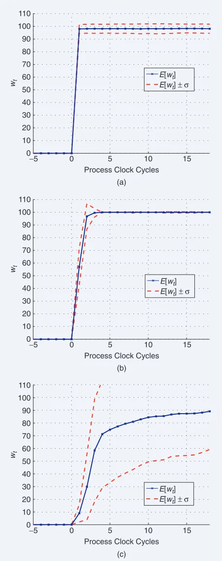
[FIG3] Expected wt ±standard deviation for λ=5. Example wtfor individual trials are also displayed. (a) Scenario A →Scenario B
(OLSR optimal). (b) Scenario B →Scenario A (DSR optimal).
−5 0 5 10 15
0 10 20 30 40 50 60 70 80 90 100 110
Process Clock Cycles wt
?
−5 0 5 10 15
0 10 20 30 40 50 60 70 80 90 100 110
Process Clock Cycles wt
?
?
(b) (a)
Trial–Specific wt E [ wt]
E [ wt] ± σ
Trial–Specific wt E [ wt]
E [ wt] ± σ
THE GIBBS SAMPLER SUPPORTS
SYNCHRONOUS AND ASYNCHRONOUS
UPDATING OF THE CHOICE OF LABEL
known a priori. A good statistic to capture the dynamic behav-ior of the framework is the percentage of nodes operating the optimal protocol, defined as
wt, at time t. There are a number of issues to consid-er such as the ability of the network to reach consensus, the length of time taken to reach such consensus, and the effect of λ on the con-vergence to consensus.
[image:8.612.67.549.76.267.2]Furthermore, we consider the whether it is possible to esti-mate an optimal value of λ.
Figure 3 shows results from the two sets of simulations. In each case the expected value for wt,E[wt], is evaluated over 100 trials and plotted against Process Clock Cyclesfor λ=5.
In both cases more than 95% of the nodes have attained the optimal protocol within five clock cycles. The dashed lines rep-resent one standard devia-tion, σ, about the mean. Majority consensus has indeed been achieved with an expected 98% of nodes on the optimal protocol. However, there is fluctua-tion between each trial run due to the random nature of the simulation, i.e., variance in local observations between sites. Examples of wtfor specific trials are also shown to illus-trate possible node behaviors and the significance of the stan-dard deviation plots. Although nodes are converging on the optimal protocol, some thrashing of protocol choice occurs in
[FIG5] Convergence statistic Dλagainst λfor each set of simulations. (a) Scenario A →Scenario B (OLSR optimal). (b) Scenario B →
Scenario A (DSR optimal).
0 20 40 60 80 100 120 140
0 50 100 150 200 250 300
λ
E[D
λ
]
0 20 40 60 80 100 120 140
0 50 100 150 200 250 300
λ
E[D
λ
]
(a) (b)
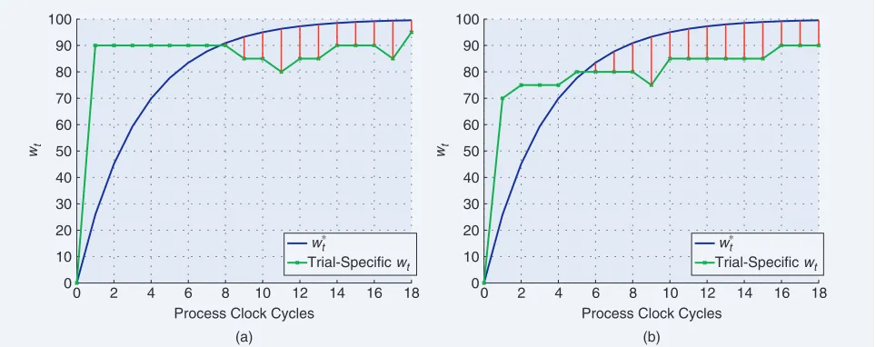
[FIG4] Target wt∗compared to realizations of wtfor individual trials. (a) Scenario A →Scenario B (OLSR optimal). (b) Scenario B →
Scenario A (DSR optimal).
0 2 4 6 8 10 12 14 16 18
0 10 20 30 40 50 60 70 80 90 100
Process Clock Cycles wt
0 2 4 6 8 10 12 14 16 18
0 10 20 30 40 50 60 70 80 90 100
Process Clock Cycles wt
(a) (b)
∗
Trial-Specific wt wt
∗
Trial-Specific wt wt
AD HOC ROUTING PROTOCOLS ARE
AT THE CORE OF AD HOC NETWORKS
AND MUST BE SPECIALLY DESIGNED
TO DEAL WITH THE DYNAMIC
individual nodes. This behavior is unacceptable as nodes on different protocols cannot communicate. Therefore, while it is important for E[wt] to converge to 100%, it is just as impor-tant for the standard deviation to converge to zero.
To capture the performance of the framework for different λ, a target convergence behavior is defined as
w∗t =100(1−exp[−ηt]). The parameter ηis chosen to yield a target of 95% of nodes converged in ten clock cycles with expo-nential convergence. wtis compared to w∗t as shown in (8) to produce the convergence statistic Dλdefined as follows.
Dλ=
t
(w∗t −wt)
I
{w∗t>wt}, (8) whereI
{w∗t>wt}=1 w∗ t >wt 0 otherwise.
Dλ is proportional to the degree with which wtis below the ideal value and is a function of λ. Figure 4(a) and (b) compares w∗t
[image:9.612.317.546.125.702.2]to trial-specific wtfor both sets of simulations. The convergence statistic Dλis equivalent to the sum of the red lines. Hence Dλis a measure of the distance of a particular experimental observation, e.g., wtin Figure 4, from the target performance w∗t. Large values of Dλimply poor convergence while small values imply perform-ance attaining our target. Note that our target is chosen as an indicative baseline measure only. The expected value for Dλ is evaluated over 100 trials for each set of simulations.
Figure 5 shows E[Dλ] against λfor each set of simulations. It shows that there is a broad range of λthat is optimal for deci-sion making and that values of λmay be chosen such that they suit both scenarios. This implies a certain amount of robustness of the system to the choice of λ. Figure 5 also shows how λ affects the overall convergence. λprovides a balance between the desire for consensus (i.e., nodes wish to operate the same protocol as their neighbors) and the need to adapt to the prevail-ing network conditions. If λis too small, then nodes do not have sufficient desire to form consensus and fragmentation of the network may take place, where different nodes operate different protocols and communication between them is lost. Nodes may also sporadically thrash between optimal and nonoptimal proto-cols due to a lack of dependence on neighboring nodes’ choices. This behavior can be seen in Figures 6(a) and 7(a) for the case where λ=0. If λis too large, the nodes do not react to chang-ing conditions, instead preferrchang-ing to form consensus with their neighbors operating the nonoptimal protocol. Again, fragmenta-tion of the network can occur. Figures 6(c) and 7(c) show this behavior at a value of λ=140. Figures 6(b) and 7(b) show the MRF-MAP performance at a value of λ=80. This value is cho-sen to be within the range of optimal λfor both simulation sets. The standard deviation tends to zero in the latter stages of simu-lation, indicating that the thrashing of protocol choice amongst nodes has abated. Thus it is possible to tune λto produce the desired global behavior in the network.
It should be noted that in these simulations, network condi-tions strongly favor either DSR or OLSR, and this is reflected in
the local observations of the nodes. The network conditions are highly stationary at all points of the network, and so nodes are likely to infer the optimal protocol from local observations alone
[FIG6]Expected wt±standard deviation. Scenario A →Scenario
B (OLSR optimal). (a) λ=0, (b) λ=80, (c) λ=140.
−5 0 5 10 15
0 10 20 30 40 50 60 70 80 90 100 110
Process Clock Cycles wt
(a)
−5 0 5 10 15
0 10 20 30 40 50 60 70 80 90 100 110
Process Clock Cycles wt
(b)
−5 0 5 10 15
0 10 20 30 40 50 60 70 80 90 100 110
Process Clock Cycles wt
(c)
E[wt] E[wt] ± σ
E[wt] E[wt] ± σ
(λ=0). However, the stochastic nature of the ad hoc networks implies that some observations may cause a node to infer the nonoptimal protocol, and it is in these cases that the framework facilitates convergence to the optimal protocol and ensures that
nodes remain on the optimal protocol. The results prove that a nontrivial choice of λleads to higher consensus among nodes and a reduction in nodes thrashing to the nonoptimal protocols. In practical terms, self-stabilizing techniques can be used to avoid thrashing once nodes have been perturbed from a suboptimal state to the optimal state using the MRF-MAP framework [23].
The MRF-MAP framework is shown to be a viable method of producing distributed consensus in ad hoc networks. The sto-chastic nature of ad hoc networks presents a challenge to the decision-making process, however appropriate selection of λ allows for quick convergence to the optimal protocol. Analysis reveals a large range of optimal λand consequently that the sys-tem is relatively robust to the choice of λ.
APPLICABILITY OF THE MRF-MAP FRAMEWORK
The MRF-MAP framework has proven to be a useful tool in net-work-wide protocol selection from the evidence of the experi-mental work described in this article. The question now arises as to its use for other network-wide decisions. There are a number of key issues to be considered here.
The first issue relates to the time dynamics of the problem at hand. Timing in the case of the MRF-MAP framework is a relative issue and very much depends on the decision to be made. If the time taken for a node to make an observation and the time taken for the framework to make a decision is so long that the network conditions have changed appreciably in the meantime, then it is not suitable.
The second issue in terms of the applicability of the frame-work is the issue of the observations themselves. In some cases there may not be a local physical manifestation of the effects of a global parameter. And in other cases, even when there is some-thing that can be measured locally, there may be no causal link between local measurements and the global conditions. In such cases the framework has no role to play but nor does any distrib-uted decision-making framework. In general, a centralized approach would be necessary.
The third issue that is important for the applicability of the framework relates to the actual implementation. This has been alluded to in the previous paragraphs in terms of the calculation of the clique potential. The implementation of the MRF-MAP framework must be carried out in such a way as to not overbur-den the network. For example nodes can actively query neigh-bors for their preferences or can opportunistically glean the information during the normal course of communication. The second option is more lightweight and less likely to overburden the network. Hence, implementation choices have an impact on the framework’s applicability.
CONCLUSIONS
The MRF-MAP framework presented in this article is a general framework for solving distributed-consensus problems in ad hoc networks. The framework has borrowed much from the field of imaging processing. Ideas from networking have found their way to the image processing domain through such techniques as graph cuts [12]. In this article ideas from image processing are finding a place in networking, thus closing the loop.
[FIG7] Expected wt±standard deviation. Scenario B →Scenario
A (DSR optimal). (a) λ=0(b) λ=80(c) λ=140.
−5 0 5 10 15
0 10 20 30 40 50 60 70 80 90 100 110
Process Clock Cycles wt
(a)
E[wt] E[wt] ± σ
−5 0 5 10 15
0 10 20 30 40 50 60 70 80 90 100 110
Process Clock Cycles (b) wt
E[wt] E[wt] ± σ
−5 0 5 10 15
0 10 20 30 40 50 60 70 80 90 100 110
Process Clock Cycles wt
(c)
The framework is attractive and elegant and through the ini-tial experiments presented here, very workable. It is clear that the use of the framework is very dependent on designing good likelihood functions and understanding the tuning parameter. Depending on the complexity of the application area this can be an arduous task, but no doubt the same can be said of its appli-cation to areas of image processing.
We are continuing the work in protocol selection and look-ing at the use of nonhomogeneous tunlook-ing parameters across the network, among other things. We are currently also expanding the applications of the framework and much can be learned from using it in different ways. Reconfigurable wireless nications systems are very much a part of the future of commu-nication systems in general and the facilitation of reconfiguration in ad hoc networks is in line with developing trends. We are particularly interested in opportunistic use of spectrum, spectrum pooling and spectrum rental for nonincum-bents. The MRF-MAP framework can aid self-organizing collabo-rative and distributed entities to make decisions about key resources in this and many other areas.
ACKNOWLEGMENT
This material is based on works supported by Science Foundation Ireland under Grant 03/CE3/I405.
AUTHORS
Linda E. Doyle ([email protected]) is a lecturer in the
Department of Electronic and Electrical Engineering, University of Dublin, Trinity College, Ireland. She leads the Emerging Networks strand of the Centre for Telecommuni-cations Value-Chain Research (CTVR). One of the main proj-ects she is currently pursuing, the Plastic Project, focuses on distributed reconfigurable and cognitive wireless networks for dynamic spectrum management.
Anil C. Kokaram([email protected]) is a senior lecturer
in the Electronic Engineering Department at Trinity College Dublin, and he is a Fellow of that same institution. He was awarded the Ph.D. in 1993 from the University of Cambridge. He has published over 70 papers in the area of image and video processing and is an associate editor of IEEE Transactions on Image Processing. He is leader of www.sigmedia.tv and has research interests in numerical techniques for Bayesian infer-ence, digital video processing, motion estimation, and visual media content analysis and manipulation.
Senan J. Doyle([email protected]) is pursuing a Ph.D. in the
area of adaptive ad hoc networking and distributed decision-mak-ing architectures within the Networks and Telecommunications Research Group of the Department of Electronic & Electrical Engineering. University of Dublin, Trinity College, Ireland. He received his first class bachelor’s degree in electronic and com-puter engineering from the University of Dublin, Trinity College, in 2003 and is an Irish Research Council scholar. He has engaged in research focusing on stationarity in ad hoc simulation, feasible link statistics for adaptive ad hoc architectures and Bayesian applications in medical imaging.
Timothy K. Forde([email protected]) is a researcher at the
Centre for Telecommunications Value-Chain Research (CTVR), Trinity College Dublin, Ireland. He received his Ph.D. degree in electronic engineering from Trinity College, Dublin, in 2005. He has engaged in various research activities focusing on mobile ad hoc networks, emerging network architectures, and dynamic spectrum access techniques. Currently, he is working on devel-oping a dynamic spectrum access platform for use in licensed Irish radio spectrum.
REFERENCES
[1] D.B. Johnson and D.A. Maltz, “Dynamic source routing in ad hoc wireless net-works,” Mobile Computing, vol. 353, pp. 153–181, 1996.
[2] P. Jacquet, P. Mhlethaler, T. Clausen, A. Laouiti, A. Qayyum, and L. Viennot, “Optimized link state routing protocol for ad hoc networks,” in Proc. IEEE INMIC’01, Lahore, Pakistan, Dec. 2001, pp. 62–68.
[3] S. Nesargi and R. Prakash, “MANETconf: configuration of hosts in a mobile ad hoc network,” in Proc. 21st Annu. Joint Conf. IEEE Comput. Commun. Soc., vol. 2, June 2002, pp. 1059–1068.
[4] N.H. Vaidya, “Weak duplicate address detection in mobile ad hoc networks,” in
Proc. 3rd ACM Int. Symp. Mobile Ad Hoc Networking & Computing, Lausanne, Switzerland, 2002, pp. 206–216.
[5] H. Attiya and J. Welch, Distributed Computing: Fundamentals and Advanced Topics. McGraw-Hill: New York, 1998.
[6] R. Guerraoui and A. Schiper, “Consenus: The big misunderstanding,” in Proc. 6th IEEE Workshop on Future Trends of Distributed Computing Syst., Tunis, Tunisia, 1997, p. 183.
[7] M.J. Fischer, N.A. Lynch, and M.S. Paterson, “Impossibility of distributed con-sensus with one faulty process,” J. Assoc. Comput. Mach., vol. 32, no. 2, pp. 374–382, Apr. 1985.
[8] L. Briesemeister and G. Hommel, “Localized group membership service for ad hoc networks,” in Proc. 2002 Int. Conf. Parallel Processing Workshops, Vancouver, BC, Canada, Aug. 2002, pp. 94.
[9] J. Besag, “On the statistical analysis of dirty pictures,” J. Royal Statistical Soc. B, vol. 48, pp. 259–302, 1986.
[10] B.S. Manjunath and R. Chellappa, “Unsupervised texture segmentation using Markov random fields,” IEEE Trans. Pattern Anal. Machine Intell., vol. 13, pp. 478–482, 1991.
[11] R.C. Dubes and A.K. Jain, “Random field models in image analysis,” J. Applied Statistics, vol. 16, pp. 131–164, 1989.
[12] Y. Boykov, O. Veksler, and R. Zabih, “Fast approximate energy minimization via graph cuts,” IEEE Trans. Pattern Anal. Machine Intell., vol. 23, no. 11, pp. 1222–1239, 2001.
[13] S. Geman and D. Geman, “Stochastic relaxation Gibbs distributions, and the Bayesian restoration of images,” IEEE Trans. Pattern Anal. Machine Intell., vol. 6, no. 2, pp. 721–741, 1984.
[14] S.Z. Li, Markov Random Field Modeling in Computer Vision.New York: Springer Verlag, 1995.
[15] Z.J. Haas, “A new routing protocol for the reconfigurable wireless networks,”
inProc. IEEE 6th Int. Conf. Universal Personal Communications, 1997, vol. 2, pp. 562–566.
[16] S.R. Das, C.E. Perkins, and E.M. Royer, “Performance comparison of two on-demand routing protocols for ad hoc networks,” IEEE Pers. Commun., vol. 8, no. 1, pp. 16–28, 2001.
[17] L. Viennot, P. Jacquet, and T.H. Clausen, “Analyzing control traffic overhead versus mobility and data traffic activity in mobile ad-hoc network protocols,” Wireless Networks, vol. 10, no. 4, pp. 447–455, July 2004.
[18] D.D. Perkins, H.D. Hughes, and C.B. Owen, “Factors affecting the perform-ance of ad hoc networks,”in Proc. IEEE Int. Conf. Commun., vol. 4, 2002, pp. 2048–2052.
[19] T.H. Clausen, P. Jacquet, and L. Viennot, “Comparative study of routing proto-cols for mobile ad-hoc NETworks,”in Proc. 2002 Int. Federation for Information Processing Med-Hoc-Net Conf.
[20] D. O’Mahony and L.E. Doyle, “An adaptable node architecture for future wire-less networks,” Mobile Computing: Implementing Pervasive Information and Communication Technologies,pp. 77–92, 2002.
[21] P. Mackenzie, “Reconfigurable software radio systems”, Ph.D. dissertation, Trinity College, Dublin, Ireland, 2004.
[22] G. Lin, G. Noubir, and R. Rajamaran, “Mobility models for ad-hoc network simulation,”in Proc. IEEE Infocom, vol. 1, Apr. 2004, pp. 454–463.