External Sector Responses to Oil Price Shocks: A Structural System Model for Nigeria

(1)

https://www.scirp.org/journal/tel ISSN Online: 2162-2086

ISSN Print: 2162-2078

DOI: 10.4236/tel.2019.98180 Dec. 11, 2019 2885 Theoretical Economics Letters

External Sector Responses to Oil Price Shocks:

A Structural System Model for Nigeria

Chukwuemeka Onyimadu

Department of Research and Training, National Institute for Legislative Studies, National Assembly Abuja, Nigeria

Abstract

This study critically examines the effects of specific exogenous shocks—oil price shocks on Nigeria’s external sector. Employing a Structural Macroeco-nomic Model (SMM) comprising of ten behavioural equations and four iden-tities with quarterly data spanning from 1981 to 2015, the SMM simulations of the external sector found that oil price shocks do have significant impacts on the components of Nigeria’s external sector. Specifically, while oil price shocks elicited varying responses from all components of Nigeria’s external sector components, the simulated results showed very limited evidence of asymmetry in the responses to both positive and negative oil price shocks. For policy, the simulated responses of capital financial flows, foreign debt flows, imports, nominal exchange rates, reserves, remittances, and capital fi-nancial flows, reflect the over-dependence of the Nigerian economy on crude oil, and the justifiable need to diversify the Nigerian economy away from the oil sector.

Keywords

Exogenous Shocks, Diversification, Macroeconomic Modeling, Economic Simulation, Uncertainty

1. Introduction

Achieving macroeconomic objectives—economic growth, full employment, price stability and balance of payments stability—remain an integral commit-ment of the Nigerian governcommit-ment and policy-makers alike. The external sector which is a subset of the general macro economy, as captured by the overall bal-ance of payments account, provides a fundamental connection between Nigeria’s dealings with the rest of the world and how actions—trade, capital flows and foreign policy—can influence Nigeria’s external sector outcomes. Indeed, to fully

How to cite this paper: Onyimadu, C. (2019) External Sector Responses to Oil Price Shocks: A Structural System Model for Nigeria. Theoretical Economics Letters, 9, 2885-2913.

https://doi.org/10.4236/tel.2019.98180

Received: September 18, 2019 Accepted: December 8, 2019 Published: December 11, 2019

http://creativecommons.org/licenses/by/4.0/

(2)

DOI: 10.4236/tel.2019.98180 2886 Theoretical Economics Letters

grasp the workings of Nigeria’s macroeconomic structure requires a detailed and thorough study of its external sector and the external sector’s role as a possible propagative channel through which exogenous shocks originating outside the economy can affect the domestic real economy. For example, developing open economies like Nigeria depend on trade, consumption of imported goods and foreign direct investments, which have direct consequences on the real, fiscal and financial sectors of its macro economy [1].

The literature on the effects of, especially, oil price shocks (demand side shocks) on the domestic economy for both developing and developed economies is vast [2] and [3]. There is ample evidence to suggest that oil price shocks do matter, as its accompanied windfall revenues may be beneficial or detrimental

[4][5]. To this end, different studies have looked into the role of oil price shocks and the uncertainty caused by oil price shocks on possible responses of selected macroeconomic variables; the effects on economic growth [6], monetary and fiscal policy responses [7][8]and financial markets [9][10].

The major problem that now exercises researchers, is not to determine if oil price shocks do matter, as that has been established from the literature. What is of utmost importance is to understand the process by which the effects of these shocks are transmitted to the domestic economy. Empirically this can be achieved by first tracing the effects of these shocks on all components of the shock transmission channel, and secondly, by eliciting the responses of domestic macroeconomic variables from the shock responses of the components of the transmission channel. The channel through which the effects of these exogenous shocks are propagated to the domestic economy is by external sector compo-nents. Addressing this problem is important because, as [11] and [12] argued, all shocks are uniquely different in characteristics and transmission. Their argu-ment was based on their findings that the transmission of oil price shocks and the responses to these shocks, depends on if the shock is a positive or negative shock, a large shock or small shock, politically motivated shock or a shock caused by nature, a demand or supply shock. Thus, a proper investigation into any form of exogenous shock will entail a critical study of its transmission channel, i.e. providing an in-depth understanding of the path through which the shock affects the real economy.

The literature on the effects of oil price shocks on the domestic economy for both developing and developed economies has been firmly established [6][11],

(3)

DOI:10.4236/tel.2019.98180 2887 Theoretical Economics Letters

rates [14], trade [15] and interest rate [16], and foreign investments [17], as possible transmission channels through which exogenous shocks are propagated to Nigeria’s real economy. Despite these limited efforts, the literature is scanty on the roles of other important external sector components, like remittances, service exports, foreign portfolio investments and external debt.

This study will provide insights into the responses of Nigeria’s external sector, which is an important transmission channel for oil price shocks. Especially in recent times, where global oil price shocks and exchange rate fluctuations are primary concerns for Nigeria, this study will provide detailed understanding on how oil price shocks affect Nigeria’s external sector and also provide policy tools for intervention. This will be beneficial to the Nigerian government, policy makers, and all economic agents that partake in the global market place. On this basis, the study sets out to 1) expand on the literature on the effects of oil price shocks. 2) Show the effects of oil price shocks on the Nigerian external sector. 3) Provide policy responses to oil price shocks as it relates to components of Nige-ria’s external sector and 4) show the existing inter-relationships between com-ponents of Nigeria’s external sector. In Section 2, the study focuses on the lite-rature review. In Sections 3 and 4, this study provides the methodology used and the results from the simulated model respectively. In Section 5, the paper presents the discussions and findings, and concludes in Section 6.

2. Literature Review

From economic literature, the empirical variations in both methods and va-riables used in macroeconomic modeling of the external sector depend on the peculiarities of the economy being modeled. Macroeconomic models of the ex-ternal sector therefore reflect the structure and dynamics of individual econo-mies. However, it has become conventional to include the major external sector variables—current account variables, capital account variables in such models as well as variables—such as, exchange rates, interest rates, capital mobility that acts as linkages to both the external sector and the real domestic economy.

The advantages of employing a macro econometric model of an economy or a sub sector cannot be over emphasized. In [18], literature on the methodological issues associated with macroeconomic modeling for a simple household and the macro economy as a whole was provided. In their book “The Econometrics of Macroeconomic Modeling”, they emphasized the role of economic theory in macro econometrics and adapting macro econometrics to developments in the real economy and academic research. [18] Noted that over the past twenty years, macro econometric modeling has taken advantage of advances in time series analysis. This has enabled the process of macro econometric modeling to expe-rience less of spurious regressions due to new inferential adaptation of inte-grated variables, often use of equations that abstract from real world dynamism, and extensive testing of specifications being performed.

(4)

modelling external sector components, however few, has provided possible ex-ogenous shocks that may influence the economy of an oil dependent country like Nigeria, [1] elicited the response of the external sector to exogenous shocks to oil prices and oil production quotas, [17]investigated the feedback effects of oil price shocks and oil productivity quota shocks on both the real and external sector. Despite the paucity of studies that focused on Nigeria’s external sector, other studies also investigated the effects of exogenous shocks to the external sector; [19] employed oil price, oil productivity quota shocks and foreign econ-omy productivity shocks for India; [20] used the same exogenous shocks as used in [19] but included a foreign interest rate shock for Rwanda. In this study, both negative and positive exogenous shocks will be used to elicit the response of ex-ternal sector components to shocks in oil price and oil production, foreign countries policy on interest and productivity shocks to major trade countries.

In [21] the external sector was modelled by the balance of payment equili-brium, BoP, where the overall balance of payment equilibrium is the sum of trade balance, B and the balance in capital account, K.

BPt=Bt+Kt

The foreign exchange curve used in the model relates domestic aggregate de-mand, Y, with the level of interest rate, r, that exists for a given exchange rate, η, and aggregate foreign demand, Yf_{. Therefore the persisting foreign exchange, e,}

can be represented as;

0 1 2 3

f r

r=α α+ Y+α Y +α e

Import demand was modeled as a function of income, lags of imports, price of imported goods and services in foreign currency terms, and the real effective exchange rates. Exports on the other hand were modeled as a function of real GDP, lags of export and the prices of exports in terms of the US dollar. [21] Si-mulated the macro economy of Bangladesh using base line forecast got from estimation of key macroeconomic variables. The study found that devaluing the local currency, raises the real exchange rate in Bangladesh. This causes an in-crease in aggregate demand and an interest rate differential that encourages cap-ital inflow.

Given the structure of the Nigerian economy as an oil importing as well as an oil exporting country, it becomes paramount to understand the relationship be-tween oil prices and Nigeria’s economic growth process as shocks to oil prices are likely to have both direct and indirect effects at the micro and macro levels of the Nigerian economy [22]. Oil price shock literature is divided on the exact and expected effects of these shocks on the economy. Some studies are of the conclu-sion that oil shocks have detrimental effects on economic performance, inflation, exchange rates and monetary variables [23][24][25]. Others are countering this postulate, instead insisting that oil price shocks may have very limited effects on economic activity [22][26][27][28].

(5)

institu-DOI:10.4236/tel.2019.98180 2889 Theoretical Economics Letters

tional structures and level of economic development [22]. Studies that concen-trated on developing economies show that oil price shocks have remained rele-vant in determining the extent of macroeconomic activities in such economies

[29]. In this study, they found that oil price shocks significantly affected output and exchange rates. Thus, a positive oil price shock will generate exchange rate appreciations which in turn can boost export earnings and drive domestic eco-nomic activities. [5] On the other hand, showed that sustained positive oil price shocks can lead to a decline in domestic economic activities for developing countries who are resource rich. Using the “Dutch Disease Syndrome”, consis-tent increases in oil prices for countries that are not well diversified, will bring about oil windfalls that induce the government to concentrate more on the sec-tor of the economy that generates these windfalls. As a result facsec-tor inputs and resources are directed to the windfall sector—which is the export sector—at the detriment of other trade sectors of the economy. This will, in the long run, lead to the de-industrialisation of the economy.

From existing literature, considerable amount of studies have focused on un-derstanding the relationship between oil price shocks and aggregate economic performance for various countries [24][27][30][31][32][33]. The literature on the effects of oil price shocks can be classified into three broad areas. First, stu-dies that focused more on the transmission mechanism and channels through which oil price effects are propagated on economic activity [34]. Secondly, stu-dies that focused on the nature of the relationship between oil price and aggre-gate economic activity: Either linear of nonlinear and symmetric or asymmetric

[27][35][36]. Lastly, studies that focused on proactive macroeconomic policies for dealing with oil price shocks [32][37].

The full effects of oil price shocks—both positive and negative—on general economic activity will depend to a large extent to what oil producers (govern-ment) do with the windfall revenue. [8] has argued that oil price shocks, through fiscal policies, affect economic performance.

[38] Carried out tests on the three leading descriptions of asymmetric and nonlinear response arising from the real price of oil to U.S. industrial production and other sector components. Their results show that estimated responses are sensitive to the estimation period and provide significant support for a nonlinear model especially prior to 1973. However, with post-1973 data only, the evidence against symmetry becomes considerably weaker. For example, at aggregate le-vels, the study failed to reject the hypothesis of symmetric responses to oil shocks, which is consistent with results by [39] for U.S. real GDP. Also, at the disaggregate level, there is strong evidence of asymmetries, especially for indus-tries that are energy intensive in production.

(6)

investigated the oil price shock of 2007-2008 and its effects on the US economy. Though oil price shocks in the US is largely driven by supply side shocks, oil price shocks of 2007-2008 were driven by strong demand. The effects of these demand driven oil price shocks were found to be similar to those of supply driven shocks. Principally, the shocks affected the purchase of domestic auto-mobiles and consumption spending which made a significant contribution to the US recession. [23] showed that increases in the price of oil has a negative impact on economic growth in Japan and China but a positive impact on Russia’s eco-nomic growth.

[39] Investigated how much real gross domestic product (GDP) respond to unanticipated changes in the real price of oil. Using censored oil price vector autoregressive models, conventional studies suggest a substantial decline in real GDP in response to unexpected increases in the real price of oil, yet no response to unexpected declines. In this study, the authors showed that these estimates are invalid using structural models that include both symmetric and asymmetric considerations. [7] Focused on how monetary authorities should react to an oil price shock. The New Keynesian literature has concluded that ensuring complete price stability is the optimal thing to do. In contrast, the paper argues that a meaningful trade-off between stabilizing inflation and the welfare relevant out-put gap arises in a distorted economy once one recognizes 1) that oil (energy) cannot be easily substituted by other factors in the short-run, 2) that there is no fiscal transfer available to policymakers to neutralize the steady-state distortion due to monopolistic competition, and 3) that increases in oil prices also directly affect consumption by raising the price of fuel, heating oil, and other energy sources. While the first two conditions are necessary to introduce a micro founded monetary policy trade-off, the third one makes it quantitatively signifi-cant. The optimal pre-commitment monetary policy relies on unobservables and is therefore hard to implement. To address this concern, the study derives a sim-ple interest rate feedback rule that mimics the optimal plan in all relevant di-mensions but that depends only on observables, namely core inflation, oil price inflation, and the growth rate of output (see [42]).

3. Methodology

(7)

consider the interdependence that exists between the equations in the system. The general form of the system model is:

(

, 1, , ,

)

, 1, , ; 1, ,

i t t t p t i it

f = y y₋ y₋ x α =µ i=  n t= T

where yt represents a vector of endogenous variables, xt is a vector of exogenous

variables and αi is a vector of parameters to be estimated in the system model.

t

 is a vector of possible serially correlated disturbance terms in the system model and f is a vector of real-valued functions. Endogenous variables are de-termined within the model while exogenous variables are dede-termined outside the model. All equations in the model have a unique endogenous variable attached to it such that, each equation in the model can be represented as:

(

, ,

)

i i i i

Y = f y x α

where yi is the endogenous variable in equation i. Any variable that is not

as-signed as an endogenous variable becomes an exogenous variable. The equations in the system model are divided into stochastic and identities. Identities are equ-ations that are expected to hold in reality while stochastic equequ-ations are those that can only hold with a random error1_{. Stochastic equations will be gotten}

from the estimation of the equations in the system model, while identities are derived from accounting relationships amongst variables.

The behavioral equations in the SMM will be estimated using ordinary least square (OLS) with the inclusions of lags for both dependent and independent variables in each behavioral equation. [43] Describes the possible use of OLS in estimating an SMM. According to [43], macroeconomic models are normally nonlinear, simultaneous and very large, thus they tend to have serially correlated error terms. However, the features of the SMM allows for the correction of these problems in modeling the SMM. From equation 3.2, the SMM provides a conve-nient way of correcting for the problem of serial correlation by treating the serial correlation coefficients as structural coefficients and transforms the equations into equations with serially uncorrelated error terms [43]2_.

Thus, the SMM used in estimating the effects of exogenous shocks on Nige-ria’s external sector components is adapted and improved upon from [1] and comprises the following behavioral equations written in their mathematical form:

(

)

0 0, ,

f

X =f P OPEC Y

, Xn= f NER Y

(

, f,Yn

)

, Xs=f Y X RER

(

, ,

)

,

(

d, , ,

)

M = f Y RER MLR RES

, RES=f RER P EDS X

(

, 0, , 0

)

,

(

, , , , , , 0

)

NER= f RES RMT IRD X M CPI TGE P

,FDI = f FDI

(

t k− ,PCGDP X, n

)

,

(

, f, , f,

)

FPI = f Y Y SMR INT N RE

, FDF= f IRD

(

,NER ,CR M Y, , f

)

,

*Stochastic equations express the endogenous variables, identities are relationships that are expected to hold in real life and do not have any stochastic characteristics.

2_Assume

1

it i it it

µ =ρ µ− + (t=2,,T) where it does not have serial correlated properties. Taking lags of this equation and subtracting it from the original equation 3.2, we get

( i, ,i i) ( i1, i1, i) it i it1 it

(8)

(

, us

)

RMT = f NER Y

On the basis of these mathematical equations, the econometric behavioral eq-uations to be estimated will be in the form of a double log equation:

Behavioral equations

( ) ( ) ( )

( )

0 0,1 1,1 0 2 2,1 2 3,1 1

4,1 0 3 1

f

t t t

t

LOGX V V LOGP V LOGOPEC V LOGY

V LOG X µ

− − − − = + + + + + ( ) ( ) ( )

0,2 1,2 2,2 2 3,2 2

4,2 3 2

f

n t n t

n t

LOGX V V RER V LOGY V LOGY

V LOGX µ

− −

−

= + + +

+ +

( ) ( )

0,3 1,3 2,3 2 3,3 4,3 3 3

s t s t

LOGX =V +V LOGY+V LOGX ₋ +V RER V LOGX+ ₋ +µ

( ) ( ) ( )

( )

0,4 1,4 2 2,4 3,4 1 4,4 3

5,4 2 4

d

t t t

t

LOGM V V LOGY V RER V MLR V LOGRES

V LOGM µ

− − − − = + + + + + + ( ) ( ) ( )

0,5 1,5 2,5 0 3,5 1 4,5 2

5,5 3 6,5 2 5

t t

LOGRES V V RER V P V EDS V LOGM

V LOGRES V LOGY µ

− − − − = + + + + + + + ( ) ( ) ( ) ( ) ( ) ( )

0,6 1,6 2,6 1 3,6 1 4,6

5,6 1 6,6 1 7,6 0 2 8,6 3 6

t t

t t t t

X M

NER V V LOGRES V LOGRMT V IRD V

V CPI V LOGTGE V P V NER µ

− − − − − − = + + + + + + + + + ( ) ( ) ( )

0,7 1,7 2 2,7 4

3,7 2 7

t n t

t

V V LOGPCGDP V

LOGFD LOGX V LOGFDI I µ − − − = + + + + ( ) ( ) ( ) ( ) ( )

0,8 1,8 1 2,8 2 3,8 4,8

5

2

6,8 2

,8 3 8

f f

t t t

t t

FPI V V Y V Y V SMR V INT

NE

V R V FPI µ

− − − − − = + + + + + + + ( ) ( ) ( ) ( ) ( ) ( ) 2 2

0,9 1,9 1 2,9 3,9 4,9

5,9 6,9 9

4

2 4

t t t

f

t t

t

LOGFDF V V V V V

V

IRD NER CR LOGM

LOGY V LOGFDF µ

− − − − − − = + + + + + + + ( )

0,10 1,10 2,10 3,10 3 10

us

t

LOGRMT=V +V NER+V LOGY +V LOGRMT₋ +µ

Identities

(

)

RER=NER∗ FCPI CPI

0 n

X =X +X

CA=X−M−INVI−Xs+CT

CF=FDI+FPI+OI

where X0 is oil exports, P0 is oil prices, OPEC represents OPEC quota and Yus

represents output from the United States of America, Xn is non-oil exports, NER

is the nominal exchange rates, Yn is non-oil GDP, Xs is service exports, X is the

value of exports, and RER is the real exchange rate, M is imports,Yd_represents

(9)

given that the nominal exchange rate is expressed in dollar terms), TGE is total government expenditure comprising both recurrent and capital expenditure, FPI represents foreign portfolio investment, Y is domestic GDP, SMR is stock mar-ket returns proxied by the returns on the All Share Index (ASI), INTf_{is interest}

rate for OECD countries, FDF represents foreign debt flow, YF_{is the income or}

foreign output proxy by OECD, CR represents the credit risk of the borrowing country proxied by the ratio of gross debt to GDP, RMT represents remittances, INVI represents investment income, CA is the current account balance, CF is capital financial flows, OI represents other investments in the capital account and CT represents the net current transfers as captured in the current account balance.

4. Results

The external sector components that are used to make up the SMM in this study comprises of ten behavioural equations—oil export, non-oil exports, service ex-ports, imex-ports, external reserves, foreign debt flow, remittances, foreign direct investments, foreign portfolio investments, and nominal exchange rates—and four identities. The behavioural equations are estimated in the model using OLS, with the amount of lags included for each variable determined by the Akaike information Criterion (AIC). The appropriate optimal lag length chosen for each variable in each behavioural equation, was done in such a way that the estimated errors for each behavioural equation will not exhibit serial correlation proper-ties. The estimates of the behavioural equation provide close estimates of the ac-tual historical data, which will be used in simulating a baseline for the mode.

4.1. Oil Export Equation

The estimated behavioural equation for oil exports in Table 1 showed the first lag of oil exports had positive sign while other lags had negative signs. For oil price and foreign income, the estimated signs were negative, unlike for OPEC oil production which showed a positive sign in the first lag and negative for subse-quent lags. There are positive feedback innovations for oil exports equation. The estimated indicated that oil prices might not immediately have effects of oil ex-ports, with this same conclusion plausible for OPEC oil production.

4.2. Non-Oil Export Equation

The estimates on non-oil export equation in Table 2 showed that previous quarter values of non-oil exports have strong links with the current value of non-oil exports. Also, non-oil output, real exchange rates and foreign country output also suggestively explain the variations in Nigeria’s non-oil exports. There are negative feedback innovations for non-oil exports equation.

4.3. Service Export Equation

(10)

Table 1. Model estimation result for oil exports.

LOG(X0) = 1.39999580363 * LOG(X0(−1)) − 0.324846615845 * LOG(X0(−2)) − 0.18190027768 * LOG(X0(−3)) + 0.0324272337436 * PO − 0.00569744857525 * PO(−1) − 0.0076016998432 * PO(−2) + 0.000218229060879 * OPEC + 0.000281155770049 * OPEC(−1) − 0.000541758175011 *

OPEC(−2) + 0.116489919066 * LOG(YF) − 0.0647384706743 * LOG(YF(−1)) − 0.060915329265 @INNOV X0 0.569689062

Source: Author’s computation from SMM.

Table 2. Model estimation result for non-oil exports.

LOG(XN) = 1.39999580363 * LOG(XN(−1)) − 0.324846615845 * LOG(XN(−2)) − 0.18190027768 * LOG(XN(−3)) + 0.0324272337436 * RER − 0.00569744857525 * LOG(YF) − 0.0076016998432 * LOG(YF(−1)) + 0.000218229060879 * LOG(YF(−2)) + 0.000281155770049 * LOG(YN) − 0.000541758175011 * LOG(YN(−1)) + 0.116489919066 * LOG(YN(−2)) − 0.0647384706743 @INNOV XN 0.8183643748

Table 3. Model estimation result for service exports.

LOG(XS) = 1.39999580363 * LOG(XS(−1)) − 0.324846615845 * LOG(XS(−2)) − 0.18190027768 * LOG(XS(−3)) + 0.0324272337436 * LOG(Y) − 0.00569744857525 * LOG(X) − 0.0076016998432 * LOG(X(−1)) + 0.000218229060879 * LOG(X(−2)) + 0.000281155770049 * RER −

0.000541758175011 @INNOV XS 0.4567353275

relationships between lags of service exports and current exports. Also, the esti-mates for real exchange rate and domestic output were found to have positive signs in explaining the variations in service exports, but total value of lags of ex-ports was found to have a negative response in explaining the variations in service exports. There are negative feedback innovations for service exports equation.

4.4. Import Equation

From economic theory, we modelled Nigeria’s imports to depend on lags of im-ports, domestic income, real exchange rates, domestic lending rates and reserves. The estimated equation in Table 4 showed inertia properties for imports, where previous period imports had causal effects on current imports. Also, domestic income suggests possible effects on the variations of imports. However, the re-sults from the estimates of domestic income did not conform to theory, where increases in consumption (via increases in domestic income) will increase the demand for imported commodities. There are positive feedback innovations for the imports equation.

4.5. Reserves Equation

(11)

Table 4. Model estimation result for imports.

LOG(M) = 1.39999580363 * LOG(M(−1)) − 0.324846615845 * LOG(M(−2)) − 0.18190027768 * LOG(YD) + 0.0324272337436 * LOG(YD(−1)) − 0.00569744857525 * LOG(YD(−2)) − 0.0076016998432 * RER + 0.000218229060879 * MLR + 0.000281155770049 * MLR(−1) − 0.000541758175011 * LOG(RES) + 0.116489919066 * LOG(RES(−1)) − 0.0647384706743 * LOG(RES(−2)) − 0.060915329265 * LOG(RES(−3)) + 0.544094953689

@INNOV M 0.4610127424

prices, external debt servicing, imports and domestic output. From the estimates of the equation in Table 5, there is evidence of negative responses of lags of re-serves in explaining current reserve levels. Also, we found that oil prices, imports and domestic output have negative effect on reserves. External debt services were found to have positive feedback in explaining the variations in reserves at all lags. There are positive feedback innovations for reserves equation.

4.6. Nominal Exchange Rate Equation

Exchange rate is a key factor in Nigeria’s external sector because it reflects changes in both the domestic and foreign country macroeconomic fundamen-tals. Based on this, we modelled Nigeria’s exchange rate with lags of nominal exchange rates [1], reserves, remittances, interest differentials, terms of trade, consumer price index, total government expenditure, and oil prices. Our esti-mates in Table 6 showed that the first lag of nominal exchange rates has positive effect on current exchange rates. Other variables showed a mixture of positive and negative effects at different levels of lags. Reserves, interest rate differentials, consumer price index and Total government expenditure all had positive effects on the nominal exchange rate. Oil prices and lags of nominal exchange rates on the other hand, have negative effects on current nominal exchange rates. There are negative feedback innovations for nominal exchange rate equation.

4.7. Foreign Direct Investment Equation

The sustained rise in FDI and its consequent importance on the Nigerian economy has been traced to economic reforms that allowed for foreign invest-ments in telecommunication, construction and the oil and Gas sectors. Thus, we modelled FDI as a function of per capita GDP, non-oil exports and lags of FDI to capture inertia effects where current FDI flows are affected by previous FDI flows. From the estimated equation in Table 7, we found inertia effects on FDI, while per capita GDP is seen to have both positive and negative effects on FDI at first and second lags respectively. However, the variable for non-oil exports showed a positive effect on FDI at first and fourth lags. FDI. There are negative feedback innovations for foreign direct investments equation.

4.8. Foreign Portfolio Investment Equation

(12)

Table 5. Model estimation result for external reserves.

LOG(RES) = 1.39999580363 * LOG(RES(−1)) − 0.324846615845 * LOG(RES(−2)) − 0.18190027768 * LOG(RES(−3)) + 0.0324272337436 * RER − 0.00569744857525 * PO − 0.0076016998432 * EDS + 0.000218229060879 * EDS(−1) + 0.000281155770049 * LOG(M) − 0.000541758175011 *

LOG(M(−1)) + 0.116489919066 * LOG(M(−2)) − 0.0647384706743 * LOG(Y) − 0.060915329265 * LOG(Y(−1)) + 0.544094953689 * LOG(Y(−2)) − 0.326038734525

@INNOV RES 2.817776461

Table 6. Model estimation result for nominal exchange rates.

NER = 1.39999580363 * NER(−1) − 0.324846615845 * NER(−2) − 0.18190027768 * NER(−3) + 0.0324272337436 * LOG(RES) − 0.00569744857525 * LOG(RMT) − 0.0076016998432 *

LOG(RMT(−1)) + 0.000218229060879 * IRD + 0.000281155770049 * IRD(−1) − 0.000541758175011 * X_M + 0.116489919066 * CPI − 0.0647384706743 * CPI(−1) − 0.060915329265 * LOG(TGE) + 0.544094953689 * LOG(TGE(−1)) − 0.326038734525 * PO + 0.089757803001 * PO(−1) + 0.312221320928 * PO(−2) − 0.626094868597

@INNOV NER 5.996407199

Table 7. Model estimation result for foreign direct investments.

LOG(FDI) = 1.39999580363 * LOG(FDI(−1)) − 0.324846615845 * LOG(FDI(−2)) − 0.18190027768 * LOG(PCGDP) + 0.0324272337436 * LOG(PCGDP(−1)) − 0.00569744857525 * LOG(PCGDP(−2)) − 0.0076016998432 * LOG(XN) + 0.000218229060879 * LOG(XN(−1)) + 0.000281155770049 * LOG(XN(−2)) − 0.000541758175011 * LOG(XN(−3)) + 0.116489919066 * LOG(XN(−4)) − 0.0647384706743

@INNOV FDI 1.695581558

those reforms targeted at equity participation, there has been increasing flows of portfolio investment to the Nigerian Economy [1]. Thus, we modelled FPI as a function of domestic output, foreign country output, stock market returns, for-eign country interest rates, and nominal exchange rates. From the estimates in

Table 8, both domestic and foreign country output have a strong significant effect in explaining the variations in FPI. While the effect for domestic output on FPI is negative, the effect of foreign output is positive in the first two lags but becomes negative by the third lag. The stock market returns variable is negative, while foreign interest rates and nominal exchange rates show positive effects in explaining the variations in FPI. There are positive feedback innovations in the foreign portfolio investments equation.

4.9. Foreign Debt Equation

(13)

[image:13.595.208.539.91.174.2]

Table 8. Model estimation result for foreign portfolio investments.

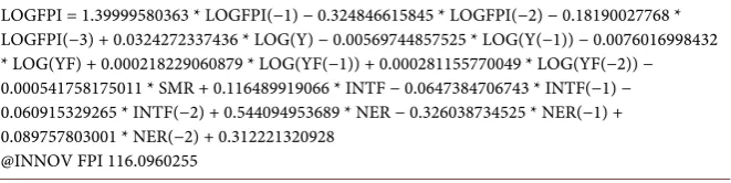
LOGFPI = 1.39999580363 * LOGFPI(−1) − 0.324846615845 * LOGFPI(−2) − 0.18190027768 * LOGFPI(−3) + 0.0324272337436 * LOG(Y) − 0.00569744857525 * LOG(Y(−1)) − 0.0076016998432 * LOG(YF) + 0.000218229060879 * LOG(YF(−1)) + 0.000281155770049 * LOG(YF(−2)) − 0.000541758175011 * SMR + 0.116489919066 * INTF − 0.0647384706743 * INTF(−1) − 0.060915329265 * INTF(−2) + 0.544094953689 * NER − 0.326038734525 * NER(−1) + 0.089757803001 * NER(−2) + 0.312221320928

@INNOV FPI 116.0960255

Source: Author’s computation From SMM.

Table 9. Model estimation result for foreign debt flow.

LOGFDF = 1.39999580363 *LOGFDF(−1) − 0.324846615845 * LOGFDF(−2) − 0.18190027768 * LOGFDF(−3) + 0.0324272337436 * LOGFDF(−4) − 0.00569744857525 * LOG(M) −

0.0076016998432 * LOG(M(−1)) + 0.000218229060879 * LOG(M(−2)) + 0.000281155770049 * LOG(M(−3)) − 0.000541758175011 * LOG(M(−4)) + 0.116489919066 * IRD − 0.0647384706743 * IRD(−1) − 0.060915329265 * NER + 0.544094953689 * NER(−1) − 0.326038734525 * NER(−2) + 0.089757803001 * CR + 0.312221320928 * CR(−1) − 0.626094868597 * CR(−2) + 11.4807096219 * LOG(YF) − 27.5395211629 * LOG(YF(−1)) + 14.4583810946 * LOG(YF(−2)) + 35.8257864344 @INNOV FDF 85.73134111

imports, nominal exchange rates, foreign country output and country risk. However, it is difficult to interpret the direction of the effects due to the changes in causal effects at different lags. Despite this drawback, the estimated results clearly show that imports, nominal exchange rates, foreign country output and lags of FDF demonstrate strong influences over the variations of FDF. There are positive feedback innovations in the foreign debt flow equation.

4.10. Remittances Equation

Remittances have become very important to the Nigerian Economy, given that it has become a viable source of foreign exchange and revenue for the government. Thus, we modelled remittances as a function of United States of America’s out-put, nominal exchange rates and lags of remittances. From Table 10, we found strong positive effects in the first lag of remittances and negative effects in sub-sequent lags, while the nominal exchange rate showed negative effects in ex-plaining changes in remittances. Output from the United States of America was estimated to have positive effects on remittances. There are negative feedback innovations for remittances equation.

4.11. Simulation Results for Within-Sample SMM

(14)

Table 10. Model estimation result for remittances.

LOG(RMT) = 1.39999580363 * LOG(RMT(−1)) − 0.324846615845 * LOG(RMT(−2)) − 0.18190027768 * LOG(RMT(−3)) + 0.0324272337436 * LOG(YUS) − 0.00569744857525 * NER − 0.0076016998432

@INNOV RMT 1.071626221

SMM against the historical data on all endogenous variables and serve as a base-line for future simulations. To achieve this, the Gauss-Seidel method uses actual values for both exogenous and lagged endogenous variables in the SMM. This is necessary because it is the within-sample simulation of the external sector com-ponents that provides a test for the reliability of the SMM given that historical data already exist for these external sector components.

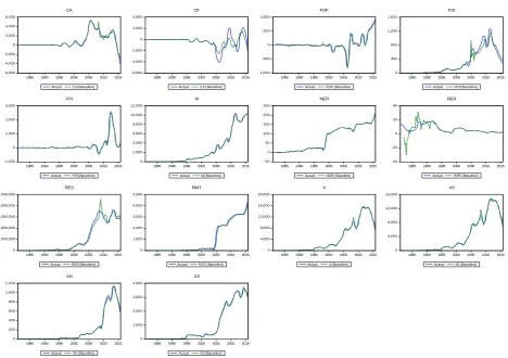
To initialise the SMM for estimating within samples, we simulate the data ad-justing the dataset to allow for the inclusion of lagged variables. Since the data ranges from 1981Q1-2015Q4, we simulate for the baseline starting from 1982Q1-2015Q1. The simulation results of the SMM showed that the simulated results for the components of Nigeria’s external sector perform well (See Figure 1). This is viewed from the simulated result’s ability to track the historical data as well as to follow the general trend and characteristics of the historical data. However, the SMM includes more fluctuations in predicting foreign debt flows and foreign portfolio investments. Despite this, the simulated results performed quite well in predicting the general trend for these two variables, making them appropriate for simulating the SMM.

4.12. Out-of-Sample Simulation Results with Exogenous Shocks

With satisfactory within-sample simulations for the SMM (See Figure 1), we provide out-of-sample simulations for the external sector components, assuming the exogenous variables experience some form of shock. With this assumption, the SMM will be able to track changes in all the external sector components. First, we have to provide a benchmark forecast of the external sector compo-nents, which will then form the yardstick for comparing simulated responses to shocks of the external sector components. Also, we introduce different scenarios to capture our assumptions of changes to the exogenous shock variables, while also assuming that the conditions within the benchmark will hold true in the future. For the different scenarios, we will track the responses of the external sector com-ponents to positive and negative changes to the exogenous shock variables—oil price, OPEC production, foreign interest rates, and foreign productivity. For the benchmark forecast of the external sector components, we assume that all com-ponents follow their trend—assume no change occurs in all variables.

4.13. Scenarios Simulation Criteria

(15)

[image:15.595.63.532.65.395.2]

Figure 1. Actual and simulated values for endogenous variables. Source: Author’s computation. The reported simulations are in the following order: CA, CF, FDF, FDI, FPI, M, NER, RER, RES, RMT, X, X0, XN, XS. All responses in this study will be ordered in this format.

assume the following scenarios to simulate both positive and negative shocks of the exogenous variables within the period 2016Q1 to 2017Q4:

Benchmark Forecast:

1) Scenario 1: All variables in the model continue on their trend path, i.e. as-sume no changes in all variables.

Exogenous shocks

2) Scenario 2: We assume that oil prices will increase to 100 dollars per barrel (pre-2015) prices and remain at that level.

3) Scenario 3: We assume that oil prices will reduce to 35 dollars per barrel and remain at that level.

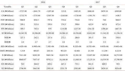
To effectively simulate these exogenous shock scenarios in the SMM, we will have to provide a benchmark forecast for the forecast and simulation range (2016Q1-2017Q4) and also for other exogenous variables in the SMM that do not comprise our shock variables (See Table 11). This is necessary as the histor-ical data for these variables ends at 2015Q4. Without providing values for 2016Q1-2017Q4 for these variables, the Gauss-Seidel method will not be able to provide accurate simulations for the endogenous variables. We solved this prob-lem by assuming s that all the exogenous variables will continue along their trend, i.e. no significant shifts in their trend and cycles and they continue in

-6,000 -4,000 -2,000 0 2,000 4,000 6,000

1985 1990 1995 2000 2005 2010 2015

Actual CA (Baseline)

CA -6,000 -4,000 -2,000 0 2,000 4,000

1985 1990 1995 2000 2005 2010 2015

Actual CF (Baseline)

CF -1,000 -500 0 500 1,000

1985 1990 1995 2000 2005 2010 2015

Actual FDF (Baseline)

FDF 0 400 800 1,200 1,600

1985 1990 1995 2000 2005 2010 2015

Actual FDI (Baseline)

FDI -1,000 0 1,000 2,000 3,000

1985 1990 1995 2000 2005 2010 2015

Actual FPI (Baseline)

FPI 0 2,000 4,000 6,000 8,000 10,000 12,000

1985 1990 1995 2000 2005 2010 2015

Actual M (Baseline)

M -50 0 50 100 150 200 250

1985 1990 1995 2000 2005 2010 2015

Actual NER (Baseline)

NER -40 -20 0 20 40

1985 1990 1995 2000 2005 2010 2015

Actual RER (Baseline)

RER 0 2,000,000 4,000,000 6,000,000 8,000,000 10,000,000

1985 1990 1995 2000 2005 2010 2015

Actual RES (Baseline)

RES 0 1,000 2,000 3,000 4,000 5,000

1985 1990 1995 2000 2005 2010 2015

Actual RMT (Baseline)

RMT 0 4,000 8,000 12,000 16,000 20,000

1985 1990 1995 2000 2005 2010 2015

Actual X (Baseline)

X 0 4,000 8,000 12,000 16,000

1985 1990 1995 2000 2005 2010 2015

Actual X0 (Baseline)

X0 0 200 400 600 800 1,000 1,200

1985 1990 1995 2000 2005 2010 2015

Actual XN (Baseline)

XN 0 1,000 2,000 3,000 4,000

1985 1990 1995 2000 2005 2010 2015

Actual XS (Baseline)

(16)

[image:16.595.60.539.90.364.2]

Table 11. Benchmark forecast for external sector components.

2016 2017

Variable Q1 Q2 Q3 Q4 Q1 Q2 Q3 Q4

CA (N billion) −3727.90 −2641.70 −1297.40 123.8 1485.20 2686.40 3659.10 4369.80 CF(N billion) −2732.70 −2735.80 −2507.50 −2143.60 −1720.40 −1301.70 −931.7 −636.7

FDF (N billion) 908.9 856.3 797.6 753.6 732.8 737.1 764 808.9

FDI (N billion) 299.1 323.4 350.4 374.3 398.6 422.9 447.6 472.4

FPI (N billion) 589.7 793.4 979 1135.80 1257.30 1341.50 1390.20 1407.70 M (N billion) 10,363.50 10,306.00 10,305.00 10,386.10 10,556.80 10,812.00 11,142.20 11,536.10

NER N 227.5 242.5 257.4 272.1 286.8 301.5 316 330.4

RER N 2.6 2.7 2.7 2.6 2.5 2.4 2.3 2.1

RES (N billion) 6.45E+06 6.90E+06 7.39E+06 7.82E+06 8.22E+06 8.55E+06 8.83E+06 9.06E+06 RMT (N billion) 1,318 484.07 203.16 90.223 42.601 21.318 11.238 6.2114

X (N billion) 7411.08 8202.28 9401.36 10,835.70 12,381.30 13,927.00 15,389.00 16,713.90 X0 (N billion) 6868.07 7637.47 8792.11 10,168.40 11,648.10 13,125.10 14,519.50 15,780.90

XN (N billion) 543 564.8 609.2 667.2 733.1 801.9 869.5 933

XS (N billion) 2796.90 2663.90 2583.10 2551.70 2583.80 2680.30 2839.10 3054.40

Source: Author’s computation. Forecast period from 2016Q1 to 2017Q4 assuming a no change in the trend of the endogenous variables. For reference, we call this Scenario 1. Deviations from this assumed path will detail the response to external sector components to exogenous shocks.

their projected paths for the periods 2016Q1-2017Q4. We first provide simula-tions for our benchmark for the external sector components for the period 2016Q1 to 2017Q4, on the assumption of no significant shifts in the trend of all the external sector components.

4.14. Oil price Shock Simulation Results

We present the SMM simulations for positive oil price shocks and then the re-sults for negative oil price shocks. In simulating the effects of oil price shocks, we assumed that the price of oil will increase to its pre-2015 levels at 100 dollars per barrel and all the other exogenous variables will continue on their trend path and not deviate from it within the time of the simulated results.

(17)

[image:17.595.58.539.90.738.2]

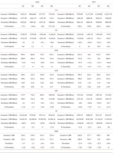
Table 12. Response of External sector components to a positive oil price shock.

2016 2017

Q1 Q2 Q3 Q4 Q1 Q2 Q3 Q4

CA

Scenario 2 (N billion) −2345.21 960.6684 4177.91 7192.58 Scenario 2 (N billion) 9750.89 11,771.90 13,258.00 14,272.70 Scenario 1 (N billion) −3727.90 −2641.70 −1297.40 123.8 Scenario 1 (N billion) 1485.20 2686.40 3659.10 4369.80

Deviation (N billion) 1382.60 3602.40 5475.30 7068.80 Deviation (N billion) 8265.70 9085.50 9598.90 9902.90 % Deviation −37.1 −136.4 −422 5711.30 % Deviation 556.5 338.2 262.3 226.6

CF

Scenario 2 (N billion) −2748.70 −2792.80 −2583.60 −2,238.20 Scenario 2 (N billion) −1823.60 −1407.10 −1033.00 −729.5 Scenario 1 (N billion) −2732.70 −2735.80 −2507.50 −2143.60 Scenario 1 (N billion) −1720.40 −1301.70 −931.7 −636.7 Deviation (N billion) −16 −57 −76.1 −94.6 Deviation (N billion) −103.1 −105.4 −101.3 −92.8

% Deviation 0.6 2.1 3 4.4 % Deviation 6 8.1 10.9 14.6

FDF

Scenario 2 (N billion) 893.1 804.9 732.7 670.7 Scenario 2 (N billion) 635.4 623 632.7 659.5 Scenario 1 (N billion) 908.9 856.3 797.6 753.6 Scenario 1 (N billion) 732.8 737.1 764 808.9 Deviation (N billion) −15.8 −51.4 −64.9 −82.9 Deviation (N billion) −97.4 −114.1 −131.3 −149.4

% Deviation −1.7 −6 −8.1 −11 % Deviation −13.3 −15.5 −17.2 −18.5

FDI

Scenario 2 (N billion) 299.1 323.5 350.8 374.9 Scenario 2 (N billion) 399.5 424.1 449.1 474.3 Scenario 1 (N billion) 299.1 323.4 350.4 374.3 Scenario 1 (N billion) 398.6 422.9 447.6 472.4 Deviation (N billion) 0.03 0.16 0.36 0.62 Deviation (N billion) 0.92 1.23 1.54 1.84

% Deviation 0.01 0.05 0.1 0.17 % Deviation 0.23 0.29 0.34 0.39

FPI

Scenario 2 (N billion) 573.7 736.3 902.5 1040.50 Scenario 2 (N billion) 1153.20 1235.00 1287.40 1313.00 Scenario 1 (N billion) 589.7 793.4 979 1135.80 Scenario 1 (N billion) 1257.30 1341.50 1390.20 1407.70 Deviation (N billion) −16 −57.1 −76.5 −95.3 Deviation (N billion) −104 −106.6 −102.9 −94.7

% Deviation −2.72 −7.2 −7.81 −8.39 % Deviation −8.28 −7.95 −7.4 −6.73 M

Scenario 2 (N billion) 10,142.60 9770.82 9375.14 9018.20 Scenario 2 (N billion) 8720.15 8486.29 8312.27 8191.05 Scenario 1 (N billion) 10,363.50 10,306.00 10,305.00 10,386.10 Scenario 1 (N billion) 10,556.80 10,812.00 11,142.20 11,536.10

Deviation (N billion) −220.9 −535.2 −929.9 −1367.90 Deviation (N billion) −1836.60 −2325.70 −2829.90 −3345.10

% Deviation −2.1 −5.2 −9 −13.2 % Deviation −17.4 −21.5 −25.4 −29

NER

Scenario 2 (N) 224.2 230.5 241.2 252.6 Scenario 2 (N) 264.9 277.7 290.7 304 Scenario 1 (N) 227.5 242.5 257.4 272.1 Scenario 1 (N) 286.8 301.5 316 330.4

Deviation −3.3 −12 −16.1 −19.6 Deviation −21.9 −23.8 −25.2 −26.4

(18)

Continued

RER

Scenario 2 (N) 2.5 2.5 2.5 2.4 Scenario 2 (N) 2.4 2.2 2.1 1.9

Deviation −0.04 −0.13 −0.17 −0.19 Deviation −0.19 −0.19 −0.18 −0.17 % Deviation −1.45 −4.93 −6.27 −7.19 % Deviation −7.65 −7.89 −7.99 −8

RES

Scenario 2 (N billion) 5.33E+06 4.87E+06 4.45E+06 4.12E+06 Scenario 2 (N billion) 3.85E+06 3.63E+06 3.44E+06 3.27E+06 Scenario 1 (N billion) 6.45E+06 6.90E+06 7.39E+06 7.82E+06 Scenario 1 (N billion) 8.22E+06 8.55E+06 8.83E+06 9.06E+06 Deviation (N billion) −1.12E+06 −2.03E+06 −2.94E+06 −3.70E+06 Deviation (N billion) −4.37E+06 −4.93E+06 −5.40E+06 −5.79E+06

% Deviation −17.4 −29.5 −39.8 −47.3 % Deviation −53.2 −57.6 −61.1 −63.9 RMT

Scenario 2 (N billion) 1,322 491.4 209.11 94.302 Scenario 2 (N billion) 45.243 23.007 12.321 6.9155 Scenario 1 (N billion) 1,318 484.07 203.16 90.223 Scenario 1 (N billion) 42.601 21.318 11.238 6.2114 Deviation (N billion) 4.47 7.33 5.95 4.08 Deviation (N billion) 2.64 1.69 1.08 0.7

X

Scenario 2 (N billion) 8829.95 11,745.70 14,545.10 17,284.10 Scenario 2 (N billion) 19,714.40 21,766.10 23,422.10 24,720.90 Scenario 1 (N billion) 7411.08 8202.28 9401.36 10,835.70 Scenario 1 (N billion) 12,381.30 13,927.00 15,389.00 16,713.90 Deviation (N billion) 1418.90 3543.40 5143.80 6448.40 Deviation (N billion) 7333.10 7839.10 8033.10 8007.00

X0

Scenario 2 (N billion) 8286.86 11,180.50 13,935.00 16,615.30 Scenario 2 (N billion) 18,978.80 20,960.90 22,548.40 23,782.90 Scenario 1 (N billion) 6868.07 7637.47 8792.11 10,168.40 Scenario 1 (N billion) 11,648.10 13,125.10 14,519.50 15,780.90 Deviation (N billion) 1418.80 3543.00 5142.90 6446.80 Deviation (N billion) 7330.70 7835.80 8028.90 8002.00

XN

Scenario 2 (N billion) 543.1 565.2 610.1 668.8 Scenario 2 (N billion) 735.6 805.2 873.7 938 Scenario 1 (N billion) 543 564.8 609.2 667.2 Scenario 1 (N billion) 733.1 801.9 869.5 933

Deviation (N billion) 0.08 0.38 0.89 1.6 Deviation (N billion) 2.44 3.34 4.22 4.98

XS

Scenario 2 (N billion) 3054.00 3140.20 3181.50 3299.20 Scenario 2 (N billion) 3487.90 3759.60 4103.20 4503.60 Scenario 1 (N billion) 2796.90 2663.90 2583.10 2551.70 Scenario 1 (N billion) 2583.80 2680.30 2839.10 3054.40 Deviation (N billion) 257.1 476.2 598.4 747.5 Deviation (N billion) 904.1 1079.30 1264.10 1449.20

% Deviation 9.2 17.9 23.2 29.3 % Deviation 35 40.3 44.5 47.4

(19)

1) Current account balance continuously increases during the forecast period by 37% and above 200% in 2016Q1 and 2017Q4 respectively.

2) Capital financial flows increase by 0.6% to 14.6% in 2016Q1 and 2017Q4 respectively.

3) Foreign debt flow decrease by 1.7% to 18.5% in 2016Q1 and 2017Q4 re-spectively.

4) Foreign direct investment increase by 0.01% to 0.39% in 2016Q1 and 2017Q4 respectively.

5) Foreign portfolio investments decrease by 2.72% to 6.73% in 2016Q1 and 2017Q4 respectively.

6) Imports decrease by 2.1% to 29% in 2016Q1 and 2017Q4 respectively. 7) Nominal exchange rates appreciate from $1:N227 to $1:N224.2 by 2016Q1 and from $1:N330.4 to $1:N304 by 2017Q4.

8) Real exchange rates also appreciates by 1.45% to 8% in 2016Q1 and 2017Q4 respectively.

9) Reserves decrease by 17.4% to 63.9% in 2016Q1 and 2017Q4 respectively. 10) Remittances increase by 0.3% to 11.3% in 2016Q1 and 2017Q4 respective-ly.

11) Total exports increase by 19.1% to 47.9% in 2016Q1 and 2017Q4 respec-tively. Oil exports also increase by 20.7% to 50.7% in 2016Q1 and 2017Q4 re-spectively, while service exports also increase by 9.2% to 47.4% in 2016Q1 and 2017Q4 respectively. However, non-oil exports increased marginally by 0.01% to 0.53% in 2016Q1 and 2017Q4 respectively.

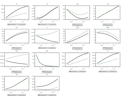
With the increase in oil prices—as captured by the positive oil price shock, Nigeria gains more in foreign exchange earnings which ultimately significantly increases her reserves and inflow of remittances. With the increases in reserves, Nigeria will be able to cover more of her imports putting less pressure on the Naira and therefore the currency appreciates in value. The simulation results show a reduction in nominal exchange rates showing that positive oil price shocks will lead to the appreciation of the Naira but imports did not increase as expected.

As expected, there was a significant increase in reserves and remittances, which seemed to be a permanent change from the benchmark. Similarly, total exports, service exports and oil exports behaved similarly with respect to their responses. Relative to total exports, service exports and oil exports, non-oil ex-ports responded with just a marginal increase (See Figure 2).

(20)

[image:20.595.62.535.58.432.2]

Figure 2. Deviations of external sector components responses to a positive oil price shock. Source: Author’s computation. The responses is captured by the bold line and the benchmark by the thinner line. Movements away from the benchmark signifies res-ponses to the Shock.

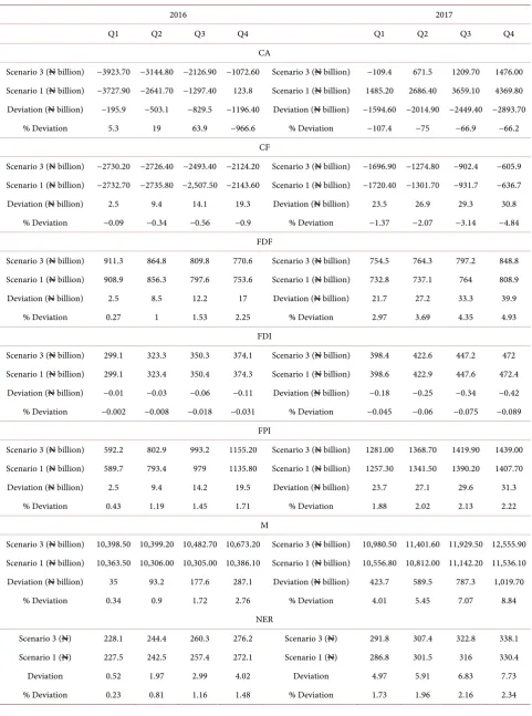
rates, reserves and remittances. A closer look at the simulation results and the percentage deviations show with a decrease in oil prices to $35, the following responses of external sector components were elicited;

1) Current account balance continuously decreases during the forecast period by 5% and above 6% in 2016Q1 and 2017Q4 respectively.

2) Capital financial flows increase by 0.09% to 4.48% in 2016Q1 and 2017Q4 respectively.

3) Foreign debt flow increase by 0.27% to 4.93% in 2016Q1 and 2017Q4 re-spectively.

4) Foreign direct investment decrease by 0.002% to 0.089% in 2016Q1 and 2017Q4 respectively.

5) Foreign portfolio investments increase by 0.43% to 2.22% in 2016Q1 and 2017Q4 respectively.

6) Imports increase by 0.34% to 8.84% in 2016Q1 and 2017Q4 respectively. 7) Nominal exchange rates depreciate from $1:N227 to $1:N228.1 by 2016Q1 and from $1:N330.4 to $1:N338.1 by 2017Q4.

-5,000 0 5,000 10,000 15,000

I II III IV I II III IV

2016 2017

CA (Scenario 2) CA (Scenario 1)

CA -3,000 -2,500 -2,000 -1,500 -1,000 -500

2016 2017

CF (Scenario 2) CF (Scenario 1)

CF 600 700 800 900 1,000

2016 2017

FDF (Scenario 2) FDF (Scenario 1)

FDF 280 320 360 400 440 480

2016 2017

FDI (Scenario 2) FDI (Scenario 1)

FDI 400 600 800 1,000 1,200 1,400 1,600

2016 2017

FPI (Scenario 2) FPI (Scenario 1)

FPI 8,000 9,000 10,000 11,000 12,000

2016 2017

M (Scenario 2) M (Scenario 1)

M 220 240 260 280 300 320 340

2016 2017

NER (Scenario 2) NER (Scenario 1)

NER 1.8 2.0 2.2 2.4 2.6 2.8

2016 2017

RER (Scenario 2) RER (Scenario 1)

RER 2,000,000 4,000,000 6,000,000 8,000,000 10,000,000

2016 2017

RES (Scenario 2) RES (Scenario 1)

RES 0 400 800 1,200 1,600

2016 2017

RMT (Scenario 2) RMT (Scenario 1)

RMT 5,000 10,000 15,000 20,000 25,000

2016 2017

X (Scenario 2) X (Scenario 1)

X 4,000 8,000 12,000 16,000 20,000 24,000

2016 2017

X0 (Scenario 2) X0 (Scenario 1)

X0 500 600 700 800 900 1,000

2016 2017

XN (Scenario 2) XN (Scenario 1)

XN 2,500 3,000 3,500 4,000 4,500 5,000

2016 2017

XS (Scenario 2) XS (Scenario 1)

(21)

[image:21.595.58.540.85.733.2]

Table 13. Response of external sector components to a negative oil price shock.

2016 2017

Q1 Q2 Q3 Q4 Q1 Q2 Q3 Q4

CA

Scenario 3 (N billion) −3923.70 −3144.80 −2126.90 −1072.60 Scenario 3 (N billion) −109.4 671.5 1209.70 1476.00 Scenario 1 (N billion) −3727.90 −2641.70 −1297.40 123.8 Scenario 1 (N billion) 1485.20 2686.40 3659.10 4369.80 Deviation (N billion) −195.9 −503.1 −829.5 −1196.40 Deviation (N billion) −1594.60 −2014.90 −2449.40 −2893.70

% Deviation 5.3 19 63.9 −966.6 % Deviation −107.4 −75 −66.9 −66.2

CF

Scenario 3 (N billion) −2730.20 −2726.40 −2493.40 −2124.20 Scenario 3 (N billion) −1696.90 −1274.80 −902.4 −605.9 Scenario 1 (N billion) −2732.70 −2735.80 −2,507.50 −2143.60 Scenario 1 (N billion) −1720.40 −1301.70 −931.7 −636.7 Deviation (N billion) 2.5 9.4 14.1 19.3 Deviation (N billion) 23.5 26.9 29.3 30.8

% Deviation −0.09 −0.34 −0.56 −0.9 % Deviation −1.37 −2.07 −3.14 −4.84 FDF

Scenario 3 (N billion) 911.3 864.8 809.8 770.6 Scenario 3 (N billion) 754.5 764.3 797.2 848.8 Scenario 1 (N billion) 908.9 856.3 797.6 753.6 Scenario 1 (N billion) 732.8 737.1 764 808.9 Deviation (N billion) 2.5 8.5 12.2 17 Deviation (N billion) 21.7 27.2 33.3 39.9

% Deviation 0.27 1 1.53 2.25 % Deviation 2.97 3.69 4.35 4.93

FDI

Scenario 3 (N billion) 299.1 323.3 350.3 374.1 Scenario 3 (N billion) 398.4 422.6 447.2 472 Scenario 1 (N billion) 299.1 323.4 350.4 374.3 Scenario 1 (N billion) 398.6 422.9 447.6 472.4

Deviation (N billion) −0.01 −0.03 −0.06 −0.11 Deviation (N billion) −0.18 −0.25 −0.34 −0.42 % Deviation −0.002 −0.008 −0.018 −0.031 % Deviation −0.045 −0.06 −0.075 −0.089

FPI

Scenario 3 (N billion) 592.2 802.9 993.2 1155.20 Scenario 3 (N billion) 1281.00 1368.70 1419.90 1439.00 Scenario 1 (N billion) 589.7 793.4 979 1135.80 Scenario 1 (N billion) 1257.30 1341.50 1390.20 1407.70 Deviation (N billion) 2.5 9.4 14.2 19.5 Deviation (N billion) 23.7 27.1 29.6 31.3

M

Scenario 3 (N billion) 10,398.50 10,399.20 10,482.70 10,673.20 Scenario 3 (N billion) 10,980.50 11,401.60 11,929.50 12,555.90 Scenario 1 (N billion) 10,363.50 10,306.00 10,305.00 10,386.10 Scenario 1 (N billion) 10,556.80 10,812.00 11,142.20 11,536.10 Deviation (N billion) 35 93.2 177.6 287.1 Deviation (N billion) 423.7 589.5 787.3 1,019.70

NER

Scenario 3 (N) 228.1 244.4 260.3 276.2 Scenario 3 (N) 291.8 307.4 322.8 338.1 Scenario 1 (N) 227.5 242.5 257.4 272.1 Scenario 1 (N) 286.8 301.5 316 330.4

Deviation 0.52 1.97 2.99 4.02 Deviation 4.97 5.91 6.83 7.73

(22)

Continued

RER

Deviation 0.006 0.022 0.031 0.039 Deviation 0.044 0.048 0.049 0.049

RES

Scenario 3 (N billion) 7.00E+06 7.00E+06 8.00E+06 9.00E+06 Scenario 3 (N billion) 1.00E+07 1.00E+07 1.00E+07 1.00E+07 Scenario 1 (N billion) 6.45E+06 6.90E+06 7.39E+06 7.82E+06 Scenario 1 (N billion) 8.22E+06 8.55E+06 8.83E+06 9.06E+06 Deviation (N billion) 195,758 430,681 743,810 1.11E+06 Deviation (N billion) 1.52E+06 1.97E+06 2.46E+06 2.98E+06

% Deviation 3 6.2 10.1 14.1 % Deviation 18.5 23.1 27.9 32.9

RMT

Scenario 3 (N billion) 1317 482.88 202.13 89.472 Scenario 3 (N billion) 42.085 20.969 11.002 6.05 Scenario 1 (N billion) 1318 484.07 203.16 90.223 Scenario 1 (N billion) 42.601 21.318 11.238 6.2114

Deviation (N billion) −0.7 −1.19 −1.03 −0.75 Deviation (N billion) −0.52 −0.35 −0.24 −0.16 % Deviation −0.05 −0.25 −0.51 −0.83 % Deviation −1.21 −1.64 −2.1 −2.6

X

Scenario 3 (N billion) 7212.28 7718.69 8648.75 9793.58 Scenario 3 (N billion) 11,041.40 12,289.90 13,465.50 14,521.40 Scenario 1 (N billion) 7411.08 8202.28 9401.36 10835.70 Scenario 1 (N billion) 12,381.30 13,927.00 15,389.00 16,713.90 Deviation (N billion) −198.8 −483.6 −752.6 −1042.10 Deviation (N billion) −1339.90 −1637.10 −1923.50 −2192.50

% Deviation −2.7 −5.9 −8 −9.6 % Deviation −10.8 −11.8 −12.5 −13.1

X0

Scenario 3 (N billion) 6669.28 7153.95 8039.65 9126.63 Scenario 3 (N billion) 10,308.70 11,488.70 12,596.90 13,589.60 Scenario 1 (N billion) 6868.07 7637.47 8792.11 10,168.40 Scenario 1 (N billion) 11,648.10 13,125.10 14,519.50 15,780.90 Deviation (N billion) −198.8 −483.5 −752.5 −1041.80 Deviation (N billion) −1339.40 −1636.40 −1922.60 −2191.30 % Deviation −2.9 −6.3 −8.6 −10.2 % Deviation −11.5 −12.5 −13.2 −13.9

XN

Scenario 3 (N billion) 543 564.7 609.1 666.9 Scenario 3 (N billion) 732.7 801.2 868.6 931.8 Scenario 1 (N billion) 543 564.8 609.2 667.2 Scenario 1 (N billion) 733.1 801.9 869.5 933

Deviation (N billion) −0.01 −0.06 −0.15 −0.29 Deviation (N billion) −0.47 −0.69 −0.92 −1.15 % Deviation 0 −0.01 −0.03 −0.04 % Deviation −0.06 −0.09 −0.11 −0.12

XS

Scenario 3 (N billion) 2758.90 2590.20 2482.40 2418.80 Scenario 3 (N billion) 2414.80 2468.50 2577.60 2736.00

Scenario 1 (N billion) 2796.90 2663.90 2583.10 2551.70 Scenario 1 (N billion) 2583.80 2680.30 2839.10 3054.40

Deviation (N billion) −37.9 −73.7 −100.7 −132.8 Deviation (N billion) −169.1 −211.8 −261.5 −318.4

% Deviation −1.4 −2.8 −3.9 −5.2 % Deviation −6.5 −7.9 −9.2 −10.4

(23)

8) Real exchange rates also depreciate by 0.23% to 2.34% in 2016Q1 and 2017Q4 respectively.

9) Reserves increase by 3% to 32.9% in 2016Q1 and 2017Q4 respectively. 10) Remittances decrease by 0.05% to 2.6% in 2016Q1 and 2017Q4 respec-tively.

11) Total exports decrease by 2.7% to 13.1% in 2016Q1 and 2017Q4 tively. Oil exports also decrease by 2.9% to 13.9% in 2016Q1 and 2017Q4 respec-tively, while service exports also decrease by 1.4% to 10.4% in 2016Q1 and 2017Q4 respectively. However, non-oil exports decrease marginally by 0.0%, 0.01% to 0.12% in 2016Q1 and 2017Q4 respectively.

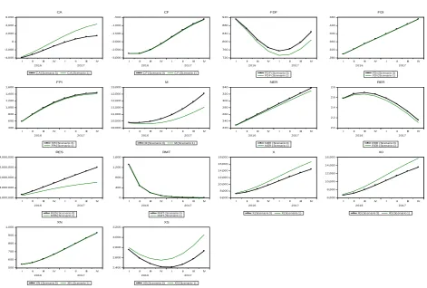
With the decrease in oil prices—as captured by the negative oil price shock, Nigeria does not gains more in foreign exchange earnings which ultimately sig-nificantly decreases her reserves and inflow of remittances. With the decrease in reserves, Nigeria will be able to cover less of her imports putting more pressure on the Naira and therefore the currency depreciates in value. The simulation re-sults show an increase in nominal exchange rates, implying that negative oil price shocks will lead to the depreciation of the Naira (see Figure 3).

5. Findings and Discussions

The simulation results from this study point to important policy implications for the Nigerian external sector. First, world oil price shocks as captured by the neg-ative and positive shocks to oil prices significantly affects the variables in the ex-ternal sector. Increases in world oil price lead to increases in capital financial flows, a reduction in foreign debt flows, while oil price reductions significantly lead to increases in imports, depreciation in nominal exchange rates, increases in reserves, reductions in remittances, and increases in capital financial flows. This reflects the over dependence of the Nigerian economy on crude oil, and the jus-tifiable need to diversify the Nigerian economy away from the oil sector.

Also, positive oil price shocks were shown to bring about decreasing responses in capital financial flows, foreign debt flow, foreign portfolio investments, im-ports, nominal exchange rates, real exchange rates and reserves. However, posi-tive oil price shocks caused substantial increases in total exports, oil exports, non-oil exports, and service exports. The simulations also show that negative oil price brought about decreasing responses in the current account balance, total exports, oil exports, and service exports. However, negative oil price shocks brought about increases in capital financial flows, foreign debt flow, foreign portfolio investments, imports, nominal exchange rates, real exchange rates, re-serves and remittances.

(24)

[image:24.595.65.537.61.379.2]

Figure 3. Responses of external sector components to a negative price shock. Source: Author’s computation. The responses is captured by the bold line and the benchmark by the thinner line. Movements away from the benchmark signifies responses to the Shock.

inflows. Since Nigeria can now cover less of her imports, we expect imports to reduce and with the loss in foreign exchange we expect the Naira to depreciate in value. The simulated results show that the Naira actually depreciates in value as the nominal exchange rate increases, but imports did not reduce as expected.

Due to the nature of the methodology used—simulations, based on assump-tions—making inferential statements on the findings of this study is not sacro-sanct. From the stated objectives of this study and the dearth in literature on studies that specifically focus on simulating external sector component’s res-ponses to exogenous shocks, making comparative assertions on external sector responses may be challenging. However, the simulated responses are discussed based on a priori expected responses that are hinged on economic intuition and economic theory. Likewise, the findings in [1] are used to check how far off the simulated responses are from the benchmarks. Although in [1], the shock as-sumptions made, scope of external sector responses, and methodology used are different from those in this study.

The output of the simulation showed that a positive oil price shock brought about significant decreases in capital financial flows, foreign debt flow, foreign portfolio investments, imports, nominal exchange rates, real exchange rates and reserves. However, positive oil price shocks caused substantial increases in total

-4,000 -2,000 0 2,000 4,000 6,000

2016 2017

CA (Sc enario 3) CA (Sc enario 1)

CA -3,000 -2,500 -2,000 -1,500 -1,000 -500

2016 2017

CF (Sc enario 3) CF (Sc enario 1)

CF 720 760 800 840 880 920

2016 2017

FDF (Sc enario 3) FDF (Sc enario 1)

FDF 280 320 360 400 440 480

2016 2017

FDI (Sc enario 3) FDI (Sc enario 1)

FDI 400 600 800 1,000 1,200 1,400 1,600

2016 2017

FPI (Sc enario 3) FPI (Sc enario 1)

FPI 10,000 10,500 11,000 11,500 12,000 12,500 13,000

2016 2017

M (Sc enario 3) M (Sc enario 1)

M 220 240 260 280 300 320 340

2016 2017

NER (Scenario 3) NER (Scenario 1)

NER 2.0 2.2 2.4 2.6 2.8

2016 2017

RER (Scenario 3) RER (Scenario 1)

RER 6,000,000 8,000,000 10,000,000 12,000,000 14,000,000

2016 2017

RES (Sc enario 3) RES (Sc enario 1)

RES 0 400 800 1,200 1,600

2016 2017

RMT (Sc enario 3) RMT (Sc enario 1)

RMT 6,000 8,000 10,000 12,000 14,000 16,000 18,000

2016 2017

X (Sc enario 3) X (Sc enario 1)

X 6,000 8,000 10,000 12,000 14,000 16,000

2016 2017

X0 (Sc enario 3) X0 (Sc enario 1)

X0 500 600 700 800 900 1,000

2016 2017

XN (Sc enario 3) XN (Sc enario 1)

XN 2,400 2,600 2,800 3,000 3,200

2016 2017

XS (Sc enario 3) XS (Sc enario 1)