Effects of spin orbit coupling and many body interactions on the electronic structure of Sr₂RuO₄

EFFECTS OF SPIN-ORBIT COUPLING AND MANY-BODY INTERACTIONS ON THE ELECTRONIC STRUCTURE OF SR_₂RUO_₄

Emil J Rozbicki

A Thesis Submitted for the Degree of PhD at the

University of St. Andrews

2012

Full metadata for this item is available in Research@StAndrews:FullText

at:

http://research-repository.st-andrews.ac.uk/

Please use this identifier to cite or link to this item: http://hdl.handle.net/10023/3217

University of St Andrews

School of Physics and Astronomy

Doctoral dissertation

Effects of spin-orbit coupling and

many-body interactions on the

electronic structure of Sr

₂

RuO

₄

.

Emil J Rozbicki

Supervisor: Dr Felix Baumberger

1. Candidates declarations:

I, Emil J Rozbicki, hereby certify that this thesis, which is approximately ... words in length, has been written by me, that it is the record of work carried out by me and that it has not been submitted in any previous application for a higher degree.

I was admitted as a research student in September 2007 and as a candidate for the degree of Philosophy Doctor in June 2011; the higher study for which this is a record was carried out in the University of St Andrews between 2007 and 2011.

Date ... Signature of candidate...

2. Supervisors declaration:

I hereby certify that the candidate has fulfilled the conditions of the Resolution and Regulations appropriate for the degree of in the University of St Andrews and that the candidate is qualified to submit this thesis in application for that degree.

Date ... Signature of supervisor ...

3. Permission for electronic publication:

In submitting this thesis to the University of St Andrews I understand that I am giving per-mission for it to be made available for use in accordance with the regulations of the University Library for the time being in force, subject to any copyright vested in the work not being affected thereby. I also understand that the title and the abstract will be published, and that a copy of the work may be made and supplied to any bona fide library or research worker, that my thesis will be electronically accessible for personal or research use unless exempt by award of an embargo as requested below, and that the library has the right to migrate my thesis into new electronic forms as required to ensure continued access to the thesis. I have obtained any third-party copyright permissions that may be required in order to allow such access and migration, or have requested the appropriate embargo below.

The following is an agreed request by candidate and supervisor regarding the electronic publi-cation of this thesis:

Access to printed copy and electronic publication of thesis through the University of St Andrews.

Contents

Abstract 7

1 Scientific Background 8

1.1 Introduction . . . 8

1.1.1 Strongly Correlated Electron Systems . . . 8

1.1.2 Fermi liquid theory . . . 9

1.2 Properties of Sr2RuO4 . . . 11

1.2.1 Crystal Structure . . . 12

1.2.2 Electronic Structure and surface reconstruction . . . 12

2 Experimental Method 15 2.1 History of Photoemission . . . 15

2.2 Kinematic description of the photoemission process . . . 16

2.3 Theoretical Principles of Photoemission . . . 19

2.3.1 Many body interactions in ARPES . . . 24

2.3.2 Matrix elements, final state effects and finite resolution effects . . . 33

2.4 Experimental Setup . . . 35

2.4.1 Getter Pumps . . . 37

2.4.2 Radiation Shield . . . 39

3 Band structure of Sr2RuO4 41 3.1 Introduction . . . 41

3.2 The Tight Binding Model . . . 43

3.3 Density Functional Theory . . . 44

3.4 Spin-Orbit Coupling in Solids . . . 47

3.5 DFT Results . . . 48

3.5.1 DFT + SOC . . . 50

3.6 TB Results . . . 51

3.6.1 Tight binding with SOC . . . 56

3.6.2 Momentum dependent Zeeman splitting . . . 57

4 Results and Discussion 61 4.1 Surface layer band structure . . . 61

4.2 Momentum dependent mass renormalization . . . 69

Abstract

The aim of the project is to investigate the effects of spin-orbit coupling and many-body interactions on the band structure of the single-layered strontium ruthenate Sr2RuO4. This material belongs to the large family of strongly correlated electron systems in which electron-electron interaction plays a crucial role in determining the macroscopic properties. The experimental method used for this purpose is Angular Resolved Photoemission Spec-troscopy (ARPES), which probes the single-particle spectral function and allows direct measurements of the quasi-particle band structure. The analysis is based on comparison of experimental data with electronic structure calculations. Typical methods for the band structure calculations including density functional theory (DFT) in the local density ap-proximation (LDA) and tight-binding calculations (TB) are one-electron apap-proximations and do not give insight into many-body interactions. However, comparing the measured band structures with calculated ones allows estimating the strength of the interactions in the considered system.

In Chapter 1 the earlier work on Sr2RuO4, which is relevant to this project is presented. This chapter is an introduction to the data analysis and discussion of the results.

In Chapter 2 we describe the experimental setup, theoretical principles of the mea-surement and summarize important improvements made during this project.

In Chapter 3 we give a brief introduction into density functional theory and describe methods used within DFT to calculate the band structure. We further give a brief de-scription of a tight binding model for Sr2RuO4. The bulk of this chapter is devoted to present the effects of spin-orbit coupling on the band structure of Sr2RuO4. In particular, we use a tight binding model to simulate the anisotropy of the Zeeman splitting found experimentally.

Chapter 1

Scientific Background

1.1

Introduction

The main subject of this thesis are many-body interactions in Sr2RuO4 probed by Angular Resolved Photoemission Spectroscopy (ARPES). This single layered strontium ruthenate belongs to the family of Strongly Correlated Electron Systems (SCES) whose macroscopic properties are dominated by the consequences of strong interactions between electrons. The layered crystal structure and two-dimensional electronic properties make Sr2RuO4 ideally suited for ARPES experiments.

According to Fermi liquid theory many-body interactions renormalize the single elec-tron bands making quasi-particles, elecelec-trons dressed by virtual excitations, heavier than bare electrons. ARPES directly measures the quasi-particle band structure - the binding energy of the many-electron states as a function of momentum. This makes ARPES a unique method to study many-body correlations as it not only provides information about the strength of the interactions but also about their momentum dependence.

1.1.1

Strongly Correlated Electron Systems

Strongly correlated electron systems continue to attract attention because of their unusual properties and extremely rich physics. Some of the intriguing states and properties of SCES are Mott insulators, heavy fermion states, colossal magnetoresistance and high temperature superconductivity. The discovery of all these effects came as a surprise and their microscopic origin is still a subject of intense debate.

Conventional band theory treats electrons as a gas of non-interacting particles moving in the fixed lattice of ions. This model works well for sp-metals such as Cu, Mg, Al, Au but breaks down for transition and rare earth elements with partially filleddandf shells. One of the most intriguing effects of electron correlations was first found in transition metal oxides. In 1937 J.H. de Boer and E.J.W. Verwey [1] reported that some of the materials predicted by the band theory to be metals are in fact insulators. As explained later by N. Mott [2] strong electron-electron interaction can induce a phase transition from the metallic to the insulating state by opening a gap at the Fermi level if the Coulomb repulsion becomes higher then the kinetic energy of the electrons.

materials is more then hundred times larger than in normal metals. As in the case of Mott insulators the effect is driven by strong electron-electron interaction. Interactions between electrons can also influence the magnetic properties of a material. A particularly distinctive example is colossal magnetoresistance. Some manganites change their resis-tivity by several orders of magnitude in a relatively weak magnetic fields because they effectively undergo a field induced metal-insulator transition. Possibly the most striking and exciting discovery related to strong correlations was high temperature superconduc-tivity in transition metal oxides. Research stimulated by this discovery led to the synthesis of a large number of new materials which revealed novel exotic phases and charge, orbital or spin ordering driven by strong correlations.

At present there is no microscopic theory that could account for all these effects. As the field of SCES is now very broad, systematic work to characterize the properties and details of many-body interactions for these materials is necessary in order to find a common denominator and lay down a basis for new theoretical treatments.

1.1.2

Fermi liquid theory

In the Sommerfeld theory of metals where interactions between electrons are neglected the ground state resulting from Pauli’s principle is a filled Fermi sea of occupied states in momentum space up to limiting wave vector kF = (3πN)

1

3 (N - density of particles in the

Fermi gas). The highest occupied state with energyF = ~ 2_k2

F

2me and momentum pF =~kF is called the Fermi level. F and pF define the Fermi surface (FS) that separates occupied

from unoccupied states. Excited states of the Fermi sea are generated by moving up electrons from states just below the FS to just above it. All excited states are uniquely labelled by the momentum quantum numbers of empty (hole) states below the FS and occupied (electron) states above it. If the interactions between the electrons are now turned on the momentum does not have to be a good quantum number anymore, rendering a description of such a system more involved. In the 1950s Landau has proposed a way around this problem. He postulated that there exists a continuous and one-to-one correspondence between the eigenvalues of the non-interacting and the interacting systems. This idea of adiabatic continuity plays a crucial role in Fermi liquid theory because it permits labeling the low energy states of the interacting system by the same quantum numbers as those of the non-interacting system as the interactions are turned on. The interactions do not change the labeling of the states, they do, however, change their energy and wavefunctions, so the particles of the interacting systems are no longer electrons but quasi-particles. The total energy of the interacting system can then be written as:

E =X k

~kF

m∗ (~k−~kF)δnk+

1 2

X

kk0

fk,k0δn_kδn_k0, (1.1)

one can evaluate the equilibrium properties of the interacting system such as specific heat

cv, magnetic susceptibility χ and resistivity ρel−el [3, 4]:

cv =

1 3

m∗pF

~3 k 2

BT, (1.2)

χ= m

∗_p

F

π2 ~

1 1 +Fa

0

µ2_B, (1.3)

ρel−el=A0

m∗2k_B2 n_~3_e2_k2

F

T2. (1.4)

The specific heat and magnetic susceptibility are very similar to their non-interacting analogs. The main difference is that they depend on the effective quasi-particle mass m∗ instead of the bare electron mass. The susceptibility has an additional term F₀a which is related to the Landau f-function and is known as Landau parameter. The effective mass is a parameter in Landau’s theory and as such has to be determined experimentally by specific heat, de Hass van Alphen or ARPES measurements. The resistivity ρel−el is

proportional to T2 in Fermi liquid theory (A0 is a dimensionless parameter and n is the electron density).

Interactions also cause a finite lifetime of the quasi-particles given by:

1

τ ∼ π

~|V| 2

g3_F2 (1.5)

where|V|2 _{is the scattering amplitude of quasi-particles, g}

F is the density of states and

is the quasi-particle energy. When is small (close to F) quasi-particles are well defined

- their lifetime is very long because the decay rate is much smaller then their energy. This no longer holds for high energies, but as long as we are concerned only with low temperatures and excitations close to the Fermi surface the quasi-particle picture is valid. Following Pauli’s principle the ground state of the non-interacting system consists of occupied states below kF and empty states above kF, so the probability of finding an

electron withk<kF is equal 1 and withk>kF is equal 0. Thus the electron distribution

function of non-interacting particles is a step function with a discontinuity atk=kF (see

figure 1.1 (a)).

1

0

kF F

1 0

z

(b)

(a)

The adiabatic continuity guarantees that the quasi-particle wavefunction will remain a fractionZ of the original non-interacting excited state wavefunction [4]:

|ψqp(k)i=

√

Z|φeli+ particle−hole excitations, (1.6)

whereZ is the overlap of an electron and q quasi-particle wavefunction and thus measures the probability of finding an electron in the quasi-particle eigenstate with momentumk. Because the quasi-particles in the interacting system contain contribution from many electrons their energy and momentum will be spread out. This translates into a step of reduced, though finite height Z < 1 at kF and some spectral weight for k > kF, i.e.

outside the non-interacting Fermi surface (see figure 1.1 (b)).

1.2

Properties of Sr

RuO

Sr2RuO4 is the single layered member of the Ruddlesden-Popper series Srn+1RunO3n+1 (where n is the number of layers). The entire series exhibits intriguing properties gen-erally attributed to many-body interactions. SrRuO3 (n = ∞) is a ferromagnetic metal with TCurie = 160 K, Sr4Ru3O10 is a ferromagnet with TCurie = 105 K that shows a

metamagnetic transition induced by magnetic field in the ab plane below 50 K. Double layered Sr3Ru2O7 is a paramagnetic Fermi liquid and shows a metamagnetic transition with a quantum critical endpoint [5, 6].

From transport measurements it is clear that Sr2RuO4 (n=1) is a paramagnetic Fermi liquid [7–10]. Figure 1.2 shows resistivity and specific heat as a function of temperature [9, 10]. The resistivity is highly anisotropic with a low temperature ratio ρc

ρab varying

Figure 1.2: Transport properties of Sr2RuO4. (a) anisotropic resistivity as a function of temperature reproduced from [9], (b) specific heat divided by temperature, filled squares in zero field open circles in 14T, reproduced from [10].

between 400 and 4000 depending on sample quality. Below 20 K the in-plane (ρab) and

interlayer resistivity (ρc) have a T2 dependence as expected within Fermi liquid theory.

38 mJ/molK2. The electronic contribution is constant below 15 K, consistent with eq. 1.2. At 1.5 K Sr2RuO4 becomes superconducting with an unusual p-wave symmetry of the order parameter and spin-triplet pairing [11].

1.2.1

Crystal Structure

Sr2RuO4 crystallizes in the K2NiF4 structure with I4/mmm body-centered tetragonal space group symmetry and is isostructural with the high temperature superconductor LaSr2−xCuxO4. In contrast to many to high temperature superconductors, Sr2RuO4 does not show any lattice distortion such as a rotation or a tilting of RuO6 octahedra or a structural phase transitions down to the lowest measurable temperatures.

Figure 1.3: Crystal structure of Sr2RuO4. (a) conventional unit cell, (b) square lattice of the RuO2 plane, (c) 3D Brillouin zone for the I4/mmm space group.

The lattice parameters measured by low temperature powder neutron diffraction are

a = 3.86 ˚A, c = 12.72 ˚A [12]. Figure 1.3 shows the crystal structure and 3D Brillouin zone of Sr2RuO4. The crystal structure is composed of alternating RuO2 and SrO2 layers. Strontium ruthenate crystals can be grown using the floating zone technique. Crystals used in this project were produced in the group of A. Mackenzie at the University of St Andrews independently by A. Gibbs and D. Slobinsky. The purity of the crystals can be characterized by the critical temperature of the superconducting state [13] which in this case was 1.52K, the highest achieved so far, indicating an outstanding quality of samples.

1.2.2

Electronic Structure and surface reconstruction

new ARPES data will be presented in Chapter 3 and Chapter 4, respectively.

The discovery of superconductivity in 1994 has moved Sr2RuO4 into the spot-light as it is the only superconducting layered perovskite without copper. Shortly after Maeno

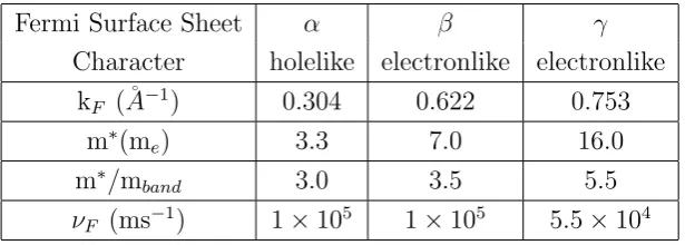
et al.[11] have reported a superconducting transition around 1 K Oguchi [14] performed band structure calculations wihin density functional theory. He found three highly two-dimensional bands at the Fermi surface. The α sheet centered at the X-point is hole-like, while the β and γ sheets are electron-like. Because of the strongly two-dimentional character of the bands, it is common to use a simplified two-dimensional Brillouin zone as shown in figure 1.4 (a). The band structure calculations were later confirmed in de Hass van Alphen (dHvA) measurements performed by Mackenzie et al. [15, 16]. These experiments further revealed a strong quasi-particle mass enhancement for all three bands as summarized in Table 1.1.

Γ α

β

γ

(a) (b)

Figure 1.4: Fermi surface of Sr2RuO4 from: (a) LDA calculations by Oguchi [14], (b) ARPES measurements by Damascelliet al. [17].

Fermi Surface Sheet α β γ

Character holelike electronlike electronlike

kF (˚A−1) 0.304 0.622 0.753

m∗(me) 3.3 7.0 16.0

m∗/mband 3.0 3.5 5.5

νF (ms−1) 1×105 1×105 5.5×104

Table 1.1: Summary of quasi-particle Fermi surface parameters of Sr2RuO4 from dHvA measurements [20].

individual contributions. Damascelli et al. [17] showed that if the sample is cleaved at

∼ 160 K the intensity of surface layer bands is substantially diminished allowing for a clearer observation of the bulk band structure. The Fermi surface from this work with all the bulk bands clearly resolved and in agreement with dHvA and LDA studies is shown in figure 1.4 (b).

Chapter 2

Experimental Method

2.1

History of Photoemission

Photoemission spectroscopy is based on the photoelectric effect discovered by Hertz in 1887 [23]. In the 1880s Hertz was working on the generation and properties of electrical oscillations. His experiments proved the existence of electromagnetic waves, predicted by Maxwell, but also revealed a new phenomenon, the photoelectric effect. Hertz noticed that metal contacts exhibit enhanced ability to spark when exposed to light. Shortly after Hertz published his results, Hallwachs observed that negatively charged plates are loosing their charge when exposed to UV light while positively charged ones do not [24]. The interpretation of these findings was far from trivial as the electron was only discovered a decade after Hallwachs’ experiments. In 1899 J. J. Thomson [25] reported the discovery of new tiny sub-particles with negative charge, later called electrons. Following work of Hertz and Hallwachs in 1902 Lenard [26] performed a series of breakthrough experiments. He measured the energy distribution of photoelectrons by applying a variable retarding potential. From the results he concluded that the number of emitted electrons depends on the intensity of the light and, surprisingly, that their velocity depends only on the light frequency. On the basis of current knowledge at the time Lenard could not explain the relationship between the maximum kinetic energy of electrons and the wavelength of the incident radiation.

In 1905 Einstein [27] proposed a phenomenological explanation of this effect. Based on Lenard’s results and formalisms derived by Planck, Wien an Boltzmann (entropy of radiation of certain frequency) he proposed that light has a particle-like nature. Its energy is distributed discontinuously in space and electrons can absorb this quanta of energy resulting in photoemission. Einstein formulated his prediction in the now famous equation for the maximum kinetic energy of the photoemitted electron

Ekin=

R

Nβν−P (2.1)

where β = h_k, k = _NR is the Boltzmann constant and N is Avogadro’s number, P is a potential step or some work done near the surface (today called the workfunction Φ).

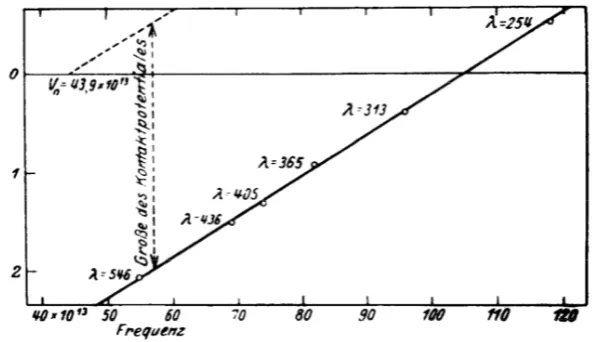
Faraday-cup technique to measure a photoelectric current as a function of wavelengths. For each frequency he observed a high-energy cutoff and, most importantly, from the fit to the experimental data got a linear dependence (figure 2.1) confirming equation 2.1.

Figure 2.1: Determination of Planck’s constant h by Millikan from the slope of electron energy versus light frequency and Einstein’s equation. Figure reproduced from [29].

Later theoretical advances came from G. Beck [30], G. Wentzel [31] and R. Oppen-heimer [32] who investigated the photoeffect and the angular distribution of electrons using formalisms from quantum mechanics.

The first use of photoemission as an analytical tool, although accidentally, was by Innes in 1907 [33]. The author investigated Pb, Zn, Ag, Pt an Au irradiated by an x-ray source. Photoelectrons of different velocity were dispersed by a magnetic field and particles were detected by photographic plates. The author emphasized the fact that the electron velocity is independent from the intensity of x-rays. However, he ascribed emitted electrons to the disintegration of atoms rather than to photoemission because of the large kinetic energy of the electrons. The first intentional x-ray photoemission study was performed by de Broglie in 1921 [34], who verified Einstein’s relation at high photon energies.

After 1950 there were two great instrumental improvements made that helped to establish photoemission as an analytical tool for the study of atoms, molecules and solids. In the early 1950s Siegbahn and coworkers built a high resolution XPS spectrometer [35, 36] and collected photoemission data for many of solids and gases [37, 38]. In 1960s D. Turner and coworkers developed the first differentially pumped helium discharge lamp, which helped to improve the resolution of UPS experiments down to∼ 20 meV [39–41].

2.2

Kinematic description of the photoemission

pro-cess

has been the study of complex systems whose macroscopic properties are a consequence of strong correlations between electrons.

Figure 2.2: Principle of the photoemission process. A sample exposed to a radiation source (UV, x-ray) emits electrons. The emitted electrons are collected, energy resolved and counted by an energy analyzer. Figure reproduced from [42].

Photoemission spectroscopy is based on the photoelectric effect, which was observed by Hertz in 1887 [23] and explained later by Einstein [27]. In the photoelectric effect an electron can be liberated from the solid by the incident photon if its energy exceeds the binding energy of the electron (EB) and the potential barrier between sample surface

and vacuum, the so called work function (Φ). Because the energy is conserved during the photoemission process one can obtain the electron’s binding energy by measuring its kinetic energy:

Ekin =hν−Φ−EB, (2.2)

where ν is frequency of the absorbed photon. Figure 2.3 presents the relation between the measured spectrum and the electron energy levels in the solid.

In order for the electron to be emitted into vacuum, the momentum conservation law must be also obeyed

kf −ki =khν (2.3)

where kf is the momentum of the photoelectron in vacuum, ki is the initial momentum

andkhνis the momentum of absorbed photon. For low photon energies its momentum can

be neglected as it is much smaller than the Brillouin zone size of typical solids. This means that the optical transition between the initial and the final bulk states can be described by a vertical transition (kf −ki = 0) or by transition between momentum-space points

connected by a reciprocal lattice vector G (kf −ki = G). Figure 2.4 illustrates the

kinematics of the photoemission process.

Figure 2.3: Relation between the electron energy levels in the solid and the measured spectrum in the single-particle picture. Electrons with binding energy EB can be excited

into vacuum Ev by photons with energy higher then EB + Φ. V0 is called the inner potential and it measures the energy between bottom of the valance band and the vacuum level Ev, as explained in text, it can be used to determine the normal component of the momentum wave vector. Figure reproduced from [43].

component of the wave vector parallel to surface is conserved:

ki,|| =kf,|| =k|| =

1

~ p

2meEkinsinθ, (2.4)

where θ is the emission angle. Determination of k⊥ which is not conserved requires

additional assumptions about the photoelectron final state. The simplest models use either band-like or free-electron final states, then, by using equations 2.2 and 2.4 the component of the wave vector perpendicular to the surface is given by

k⊥ =

1

~ p

2me(Ekincos2θ+V0), (2.5)

whereV0 is the inner potential of the crystal, which can be determined experimentally. Equations 2.2, 2.4 and 2.5 relate the measured kinetic energy as a function of emission angle of the photoelectronEkin(θ) to the binding energy as function of momentum of the

electron in the solid E(k) − the band structure.

description within the so-called three-step model in which the process is decomposed to three independent events: photo-excitation of the electron, travel of the photoelectron to the surface and escape into the vacuum.

Figure 2.4: Photoemission within the three-step model: (a) optical transition in the solid, (b) free−electron final state in vacuum, (c) probed photoelectron spectrum(from [44]).

2.3

Theoretical Principles of Photoemission

From a theoretical point of view, the photoemission process is an optical transition be-tween initial and final states described by many-body wave functions. The initial state is an N-electron eigenstates and the final state is an (N −1)-electron system plus the photoelectron. Fermi’s Golden Rule is a convenient and starting point to describe the photoemission process

wif =

2π

~

|hΨf|H0|Ψii|2ρf, (2.6)

wherewif is the probability of a transition between initial and final states of the system

described by the wave functions |Ψi/fi, H0 is the perturbation that caused the transition

and ρf is the density of final states. The above formula can be rewritten in the following

way to calculate the probability of photoexcitation of the N-electron groundstate|Ψiito

one of the possible excited final states|Ψficonsisting of a photoelectron with momentum kand energy Ekin = ~k

2

2me and the remaining (N −1)-electron system

wif =

2π

~

|hΨf|HP E|Ψii|2δ(f −i−hν), (2.7)

wherei/f denotes the energy of the initial and final states andHP E describes the

interac-tion with the photon. The latter can be obtained by the transformainterac-tion of the momentum operator to include the electron’s interaction with an electromagnetic field p→p− e

Starting from an unperturbed HamiltonianH0 = p

2

2me +eV(r) one gets

H = _2m1

e p−

e cA

2

+eV(r)

= ₂p_m2 e −

e

2mec(A·p+p·A) +

e2

2mec2A

2_{+eV (r)}

=H0+HP E,

(2.8)

where

HP E =−

e

2mec

(A·p+p·A) + e 2

2mec2

A2. (2.9)

Here, p is the momentum operator and A is the electromagnetic vector potential. By choosing an appropriate gauge, the scalar potential Φ can be set to zero. The quadratic term can be omitted as it is relevant only for very high intensities of the exciting radiation. Using the commutation relation [p,A] =−i_~∇·Aand the dipole approximation∇·A= 0 one gets

HP E =−

e mec

A·p. (2.10)

The dipole approximation assumes thatAdoes not change over atomic distances. This is true for the bulk. However, at the surface the electromagnetic field may vary over short length scales. This can result in asymmetric lineshapes for direct transitions. However, the effect is generally small and will be neglected here.

Figure 2.5: One-step model vs three-step model. The three-step model consists of (1) photoexcitation of an electron, (2) travel to the surface and (3) transmission through the surface into vacuum. In the one-step model an initial state electron is excited into a wave that propagates freely in vacuum but decays away from the surface into the solid (from [46]).

Step one - Photoionization

This process contains all the information about the electronic structure of the solid and it is described within the so calledsudden approximation, where the interaction between the photoelectron and the remaining (N−1)−particle system is neglected. This allows to write the final state wave function as a product of the wave functions of the photoelectron

|φk,fi and an excited state s of the (N −1)−electron system |ΨNs−1i

|Ψfi=a|φk,fΨNs −1i, (2.11)

where a is an antisymmetric operator. The total transition probability is simply a sum over all excited states s. The sudden approximation holds only for electrons with high kinetic energy for which the escape time is much shorter than the system response time. In the oppositeadiabatic limitof slow electrons, the wave functions cannot be factorized and one has to include the screening between photoelectron and photohole. Using factorized forms for the wave functions the matrix elements between initial and final state can be written as

hΨf|HP E|Φii=hφk,f|HP E|φk,iihΨNs−1|ck|ΨNi i (2.12)

where ck is the annihilation operator for an electron with momentum k. The total pho-toemission intensity measured as a function of the kinetic energyEkin at a momentum k

is equal to

I(k, Ekin) =

2π

~ X

f i

|Mk,f,i|2

X

s

|cs,i|2δ Ekin+sN−1−Ni −hν

where N_s −1 is the energy of the eigenstate s of the (N −1)-electron system, |Mk,f,i|2 =

|hφk,f|HP E|φkii|2is the photoemission matrix element describing the transition probability

of a single electron from state |φk,ii to the final state |φk,fi and |cs,i|2 =|hΨNs−1|ck|ΨNi i|2

is a probability that the removal of the electron from stateiwill leave the (N−1)-electron system in the excited state s.

Step two - Transport

During the transport to the surface electrons undergo elastic and inelastic scattering. Elastic scattering is important only at high electron energies and the high incident photon energies. The inelastic processes give rise to a continuous background in the measured spectra which is usually subtracted or simply ignored. As a result of inelastic scattering electrons lose kinetic energy by exciting secondary electrons, plasmons and phonons. This limits the escape depth of photoelectrons, described byλ, the so-called inelastic-mean-free path (IMFP). The number of emitted electrons depends on the distance d they have to travel in the solid to reach the surface. The intensity of the emitted electrons is given by

I(d) =I0e −d

λ , (2.14)

where I0 is proportional to the number of the excited electrons. The energy dependence of λ is described by the so-called ”universal curve”.

Figure 2.6: The inelastic electron mean-free path in solids - “universal curve”. Figure reproduced from [46].

Step three - Escape

The only electrons that can escape from the sample are those with a component of the kinetic energy normal to the surface sufficient to overcome the surface potential barrier. Inside the crystal electrons travel in the inner potential of depthV0 =Ev−E0 (see figure 2.3), where Ev is the work function, and E0 is the bottom of the valence band. In order to escape the electron must fulfill the condition:

~2 2me

k_⊥2 ≥V0. (2.15)

wherek⊥ is the component of the wave vector normal to the surface.

During the escape of electrons to the vacuum, only the parallel component of the wave vector is conserved modulo a reciprocal lattice vector (due to the periodicity of the lattice potential parallel to the surface). Therefore, one can connect the measured kvac

k with

kcryst_k

kvac_k =kcryst_k −Gk, (2.16)

where Gk is a reciprocal lattice vector. Figure 2.7 shows the relation between vacuum

Figure 2.7: Momentum relation at the solid-vacuum interface in angle-resolved photoemis-sion. In the transmission across the crystal-vacuum interface only the parallel component of momentum is conserved, modulo a reciprocal surface lattice vector, but the normal component is altered by the surface potential.

and solid momenta. One can expressk_kcryst via the kinetic energy and the emission angle

θ with respect to the surface normal by

k_kcryst= r

2me

~2 Ekinsinθ. (2.17)

The Bloch eigenstates inside the sample have to match the free−electron plane waves in vacuum in order for the transmission to take place. The wavefunction of the final state within the solid with energy Ef(k) is given by

φf(k) =

X

G

Photoelectrons can escape from the crystal in a number of possible directions given by eq. 2.17. All planewave components of the Bloch state with the same value of kk +Gk

will leave the crystal in the same direction giving rise to the coherent beam. The total transmission factorT(Ef,kk)

2

for a given value of kk+Gk at a particular final stateEf

is given by

T(E_f,kk)

2

=t(E_f,kk+Gk)

2 X

(k+G)⊥>0

uf(G,k)

2 (2.19)

where the sum goes over all components propagating towards surface. The reduced trans-mission factort(Ef,kk+Gk)

2

which neglects surface scattering is given by

t(Ef,kk+Gk)

2 =     

1 if Ekin> ~ 2

2me(kk+Gk) 2

0 if Ekin≤ ~ 2

2me(kk+Gk) 2

(2.20)

whereEkin is electron kinetic energy in the vacuum.

As it was already mentioned, the wavevector component perpendicular to the surface is not conserved during the escape. One way around this problem is to study two dimensional systems where k⊥ does not matter. If, however, one is interested in solids with three

dimensional electronic structure there is an experimental approach that allows one to estimatek⊥. By measuring photoelectrons emitted along the surface normal as a function

of photon energy one can deductV0 in equation 2.5 from the periodicity of the measured

E(k⊥).

2.3.1

Many body interactions in ARPES

ARPES spectra can also be described within the Green’s function formalism. The propa-gation of a particle through a many-body system is described by the time ordered Green’s function. In the spectral representation the removal of an electron from the N-particle system atT = 0 is given by the following Green’s function

G−(k, ) = X

s

|hΨN_s −1|ck|ΨNi i|2

−N−1

s +Ni −iη

(2.21)

where η is small and positive. In the limit of η → 0+ _{the one-electron removal spectra} which can be measured by photoemission is given by a one-particle spectral function

A−(k, ) = −1

π=m G

− _{k, −iη}+

=X

s

hΨN_s−1|ck|ΨNi iδ − N−1

s − N i

(2.22)

For finite temperatures and within the sudden approximation the intensity of the ARPES spectrum is given by

I(k, ) =I0(k, hν,A)A(k, )f(), (2.23)

The effect on the Green’s function from many-body interactions can be described by the complex self-energy:

Σ (k, ) = <eΣ (k, ) +i=mΣ (k, ), (2.24) which contains contribution from all many-body processes (electron, electron-phonon, electron-impurity, etc.)

Σ (k, E) = Σel−el(k, ) + Σel−ph(k, ) + Σel−im(k, ) +... (2.25)

The Green’s and spectral functions in terms of self energy are given by

G(k, ) = 1

−0_{(k)−Σ (k, )} (2.26)

and

A(k, ) = 1

π

=mΣ (k, )

(−0_{(k)− <eΣ (k, ))}2_{+ (=mΣ (k, ))}2, (2.27) where0_{(k) is the single-particle dispersion which can be approximated by band structure} calculations.

For paramagnetic metals the contribution to the self energy comes mainly from the electron-electron, electron-phonon and electron-impurity interaction. In the following sections we will present model self-energies used later in the analysis of the data. In general any many-body process will have two effects on the observed spectrum. First, the position of the peak will be shifted by<eΣ (k, ) (mass renormalization) and second, peaks will gain a finite width given by 2=mΣ (k, ) (quasi-particle lifetime).

M pm en tum

(a)

(b)

Figure 2.8: (a) Spectral function for a simple cosine band, (b) corresponding energy distribution curves.

If the electrons do not experience any interactions, i.e. Σ (k, ) = 0, the Green’s function

G0(k, ) = 1

has one pole for eachkand the spectral function

A0(k, ) = 1

πδ −

0_(k)

, (2.29)

consists of a delta peak centered at the single-electron energy 0_{(k). Figure 2.8 shows} the spectral function for a simple band with cosine dispersion 0_{(k) ∝ cos (k) in the} absence of interactions. The left panel is a probability map of the energy as a function of momentum and the right panel shows energy distribution curves (EDCs) for differentk.

Electron-electron interaction

The spectral function for the general interacting system is given by equation 2.27. If

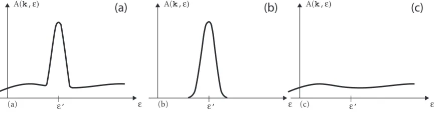
=mΣ (k, )(−0(k)− <eΣ (k, )) the spectral function A(k, ) is a Lorentzian peak of width 2=mΣ (k, ) centered at 0(k) = 0(k) +<eΣ (k, ) sitting on the background created by the continuum of the particle−hole excitations, as illustrated in figure 2.9. Because the spectral function describes the probability of adding or removing an electron with momentum kand energy it has to fulfill the sum rule:

Z +∞

−∞

dA(k, ) = 1. (2.30)

Using the above sum rule one can split the spectral function (and Green’s function) into a part that describes the coherent quasi-particle peakAc and the incoherent background

Ainc

A(k, ) = Z(k)Ac(k, ) + (1−Z(k))Ainc(k, ). (2.31)

Z(k) is called the quasi-particle weight and measures the overlap between electron and quasi-particle wavefunction. From the sum rule 2.30 Z(k) < 1, which reflects the fact that the quasi-particle state is not an isolated state but an integral part of the coupled system.

ε’ A(k,ε)

ε

ε’ A(k,ε)

ε _ε’

A(k,ε)

ε

(a) (b) (c)

(a) (b) (c)

Figure 2.9: Separation of the spectral function (a) into quasi-particle peak centered at 0

(b) and particle−hole background (c).

G(k, ) = 1

−0_(k)−∂<eΣ(k)

∂ |=(k)−i=mΣ(k)

+background

= Z(k)

−0_(k)−iΓ(k) + (1−Z(k))Ginch(k, ) (2.32)

from the definition of the spectral function 2.22:

A(k, ) = 1

π

Z(k)Γ(k)

(−0_(k))2_{+ (Γ(k))}2 + (1−Z(k))Ainch(k, ), (2.33)

where

Z(k) = 1− ∂<e_∂Σ(k)|=(k)

−1

, 0(k) =Z(k)0(k), Γ(k) =Z(k)=mΣ(k). (2.34)

The poles of the Green’s function for the interacting electron system have the energy (mass) renormalized by the factor Z(k) and a finite width (lifetime). The quasi-particles can then be viewed as electrons dressed in the virtual excitations that move with them coherently. The incoherent part of the quasi-particle is hard to define rigorously as the coherent part already contains some of the low-lying excitations.

In the Fermi liquid regime Z(k) > 0 the quasi-particle peak at the Fermi level is infinitely sharp, and its spectral weightZ(kF) is proportional to the mass renormalization m0

m∗, where m

∗ _{is the effective mass and m}

0 is the single-electron band mass. If the band dispersion is linear in the vicinity ofF the renormalization constant is given by the ratio

of the single-electron to the quasi-particle Fermi velocity (band slope at the Fermi level)

Z(kF) =

v0

F

v_F∗. (2.35)

The self−energy for the 3D Fermi liquid system is

Σel−el(, T) = α+iβ2+ (πkBT)2

. (2.36)

The coherent part of the spectral function is then given by

A(k, ) = 1

π

β02

(−0_(k))2_+β024, (2.37)

where

Z(kF) = ₁₋1_α, 0(k) = Z(kF)0(k), β0 =Z(kF)β. (2.38)

Mom

entu

m

(a)

(b)

Figure 2.10: (a) Spectral function of the three dimensional Fermi liquid, (b) EDC’s from panel (a). The red line is the non-interacting band.

Electron-phonon interaction

The interaction between electrons and lattice vibrations can strongly affect quasi-particle energies close to the Fermi level. In general the interaction of an electron with bosonic modes (phonons, magnons, plasmons, etc.) leads to two effects: an enhancement of the quasi-particle mass and a so called ”kink” - a sudden change of the slope of the band at an energy characteristic for the given interaction (e.g. the Debye temperature for phonons).

The spectral function for the electron-phonon system is given by

A(k, ) = 1

π

Zel−ph_(k)Γel−ph_(k)

(−0_(k))2_{+ (Γ}el−ph_(k))2, (2.39)

where Γel−ph(k) =Zel−ph(k)=mΣel−ph(k, ) and Zel−ph(k) is the electron−phonon renor-malization constant given by

Zel−ph(k) =

1−∂<eΣ

el−ph_(k)

∂

=(k)

!−1

. (2.40)

The electron−phonon interaction can be described by the Eliashberg functionα2F(_~ω), whereF (_~ω) is the phonon density of states and α is the electron−phonon coupling pa-rameter. The self−energy for the electron−phonon interaction is given by [47]

Σel−ph_{(k, , T) =}R

d0R~ωmax

0 d(~ω)α 2_F(

~ω)

×h1−f(0,T)+n(~ω,T)

−0₋

~ω +

f(0,T)+n(~ω,T)

−0₊

~ω

i

,

(2.41)

For the imaginary part of Σel−ph one gets

=mΣel−ph_{(k, , T) = π}R~ωm

0 α

2_{F (}0₎

×[1 + 2n(0) +· · ·+f(+0)−f(−0)]d0.

(2.42)

Debye model

In the Debye model the maximum phonon energy is given by the Debye energy _~ωD.

The dispersion of phonon modes in three dimensions is linear, _~ω ∝ k, and only the longitudinal modes interact with the electrons withα(ω) =const.. Hence, the Eliashberg function is proportional to the density of phonon levels and is given by

α2F() =        λ

~ωD 2

, ≤_~ωD,

0, >_~ωD,

(2.43)

where λ is the mass-enhancement factor, and is defined by the change of the electronic group velocityvk= 1_~δδ_k which changes by a factor of Zel−ph(k) = ₁₊1_λ close to the Fermi level (the electronic density of states and the band mass increase by a factor of (1 +λ)). From eq. 2.40 we get the connection between λ and the real part of the electron-phonon self-energy

λ=− δ<eΣ

el−ph₍₎

δ

=F

, (2.44)

The mass-enhancement factor is anisotropic and temperature dependent. It decreases withT and vanishes at high temperatures. The effect of mass renormalisation by electron-phonon coupling can be observed for various physical properties such as the electronic heat capacity at low temperatures, the cyclotron effective massmc in the de Hass-van Alphen

effect, or the Fermi velocity. However, the shape of the Fermi surface remains unchanged.

λ is given by he first moment of the Eliashberg coupling function at T = 0:

λ=

Z ~ωmax

0

α2_F( ~ω) ~ω

d(_~ω). (2.45)

In the limit of high temperatures, one gets a linear dependence of the imaginary part and the photoemission linewidth on the temperature

=mΣel−ph(T) = Γ

el−ph_(T)

2 =πλkBT, kBT ~ωD. (2.46)

In the limit of T = 0 one gets an analytical description for the energy dependence of the real and imaginary part of the self-energy

=mΣel−ph() = Γ

el−ph₍₎

2 =      π 3λ 3

(~ωD)2, ≤~ωD,

π

3λ~ωD, >~ωD.

5 4 3 2 1 0

E/h

ω

0 0.25 0.5 0.75 1

real part of

Σ

el-ph

/

Σ

D T = 0.5θ_D

5 4 3 2 1 0

E/h

ω

1 2

imaginary part of

Σ

el-ph

/

Σ

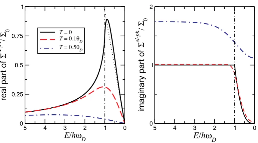
Figure 2.11: Plots of the energy dependence of the self−energy in the Debye model for

λ= 1. Panel (a) gives the real part of the self-energy and panel (b) shows the imaginary part of the self-energy. θD is the Debye temperature, ~ωD is the Debye energy and

Σ0 = π₃λ~ωD is the normalization constant. Figure reproduced from [46].

and

<eΣel−ph_{() = −λ}~ωD 3

~ωD

+

~ωD 3

ln

1−

~ωD

2 + ln 1+ ~ωD 1− ~ωD . (2.48)

The real part<eΣel−ph_{and imaginary part=mΣ}el−ph_{of the self energy are presented in}

figure 2.11. The real part increases linearly fromF and shows a maximum at the Debye

temperature ~ωD

kB . Increasing the temperature shifts the maximum to higher binding energies and decreases the value of <eΣel−ph. The imaginary part at T = 0 has a sharp edge at_~ωD that smears out with increasing temperature.

Figure 2.12 shows the spectral function of a simple cosine band 0_{(k)∝ cos (k) with} electron-photon interaction. Panel (a) and (b) presents a gray scale plot and stack of EDCs, respectively. As one can see, below the Debye temperature || > _~ωD, the band

has the original single-electron dispersion while above it,||<_~ωD, the electron dispersion

is renormalized byZel−ph(k) = ₁₊1_λ.

In figure 2.13 (b) we show three EDCs from the electron-phonon spectral function. One intersecting the band at its bottom (black line), one at the Fermi level (blue line) and one at the Debye energy (red line). These EDCs reveal that the spectra are actually composed of two different branches. For binding energies above the Debye temperature

|| _~ωD the electron modefollows the original single-electron dispersion and the

quasi-particle peak has a constant width and intensity. For || _~ωD the phonon mode has

Mom

en

tum

(a)

(b)

Figure 2.12: (a) Spectral function and (b) EDC stack for a cosine band coupled to phonons described by a Debye model. The red line denotes the non-interacting band.

approaching the Fermi level. Exactly at the Fermi level (for T = 0) the quasi-particle peak reaches its maximum height and is infinitely sharp. In the cross-over region for

|| ∼ _~ωD, there is a transition from an electron mode to a phonon mode, the spectral

weight of these two features gets comparable in this region and the quasi-particle peak is not well defined anymore. All spectra exhibit a characteristic three peak structure. In particular the cross-over region has rather complex structure due to the fact that both branches approach each other with similar spectral weight. For the states far away from the cross−over region (black and blue EDCs), the two incoherent features, located at

||=_~ωD have low spectral weight compared to the coherent part, however, they do not

vanish.

Due to the complex shape of the spectral function, the peak positions from EDCs and MDCs for the electron-phonon coupled system differ substantially, as shown in figure 2.13 by red and green lines. While EDCs show three peak structure, and hence existence of two different branches, the MDCs are always composed of a single Lorentzian peak. This means that the MDC dispersion can be described by a single line (red line in figure 2.13 (a)) that shows a kink at||=_~ωD, where the dispersion changes from the unrenormalized

to the renormalized band.

Momentum Distribution

(a)

(b)

Figure 2.13: (a) Spectral function for an electron-phonon coupled system reproduced from figure 2.12 (a). The green line gives the peak position of the EDCs. Interaction splits the band into two branches, anelectron modebelow Debye temperature and a phonon mode

above it. The red line shows the peak position fitted from MDCs and the kink in the dispersion visible at the Debye temperature. Panel (b) shows three representative EDCs. Black− band bottom, Blue− Fermi level, Red − cross-over region.

that the spectral weight is smeared over many states results in a reduced discontinuity at the Fermi level in the momentum distribution function n(k) even at T = 0. The momentum distribution is given by

Z +∞

−∞

df()A(k, ) =n(k). (2.49)

wheref() is the Fermi distribution function. The size of the discontinuity is given by the total renormalization resulting from electron-electron and electron-phonon interaction. For a Fermi liquid coupled to a Debye spectrum of phonons:

Ztot(kF) =

1

1− ∂<eΣel−el

∂

=F

− ∂<eΣel−ph

∂

=F

= 1

1−α+λ. (2.50)

In the non-interacting system the discontinuity at the Fermi wave vector kF defines the

Fermi surface−there are no states outside the Fermi surface. In the case of the interacting system there is a finite occupation probability even for states withk>kF. However, for

a Fermi liquid the discontinuity is always finite (Z >0) so one can still identify the Fermi surface by locating the maxima of|∇kn(k)|.

Figure 2.14: Momentum distribution for the interacting system. The step size is given by the total renormalization resulting from electron−electron and electron−phonon interac-tion [46].

2.3.2

Matrix elements, final state effects and finite resolution

effects

In a real experiment the extraction of quantitative information from ARPES data is further complicated by effects of matrix elements, finite experimental resolution and due to the background of secondaries. The total measured intensity can be then written as

I(k, ) = [I0(k, hν,A)f()A(k, ) +B]⊗[R(∆)Q(∆k)], (2.51)

whereB is the background,R(∆) is the energy andQ(∆k) is the momentum resolution function and ⊗ denotes the convolution. The convolution leads to mixing of momentum and energy space. Momentum resolution affects not only MDCs but also EDCs and vice versa. There is no easy way around this problem. Standard deconvolution techniques do not work for ARPES data and full 2D fitting demands a large number of parameters. So usually there are some simplification applied to the fitting procedure.

I0(k, hν,A) ∝ |Mf,i(k)|2 for simplicity of the data analysis is usually assumed to be

unity, however, this term may have a strong effect on the measured photocurrent and can even lead to the complete suppression of the intensity. It depends on the photon energy, polarization and experimental geometry.

The matrix elements are proportional to the overlap between initial and final state wavefunction

|Mk,f,i|2 ∝ |hφk,f|A·p|φkii|2 (2.52)

The matrix element will be nonzero only if the product of terms in the overlap integral is even function with respect to the mirror plane. The final state wavefunctionφk,f must be

the dx2_−y2 orbital which is even. Hence, the photoemission process is symmetry allowed

only forA even (p- polarization).

Figure 2.15: Mirror plane emission from ad_x2_−y2 orbital. Figure reproduced from [44].

Another complication that may arise in the interpretation of ARPES data is that the experimental linewidth contains contributions from the photohole (initial state) and pho-toelectron (final state). The spectral function derived in the previous section describes only the initial state of the system. However, the contribution to the spectra from the fi-nal states can be quite large and complex. In general it can be described by a convolution of the spectral function of the photohole with the spectral function of the photoelec-tron. In the case of a weakly interacting system, the contributions from photohole and photoelectron can be described by Lorentzians with linewidths Γi (photohole) and Γf

(photoelectron). The resulting linewidth Γm is a linear combination of these two, given

by

Γm =

Γi

|vi⊥| + Γf

|vf⊥| 1 vi⊥

1−mvi||sin2θ

~k||

− 1

vf⊥

1− mvf||sin2θ

~k||

, (2.53)

where_~v(i,f)⊥=δ/δk⊥. For normal emission (θ = 0◦) and with |vi⊥| |vf⊥|

Γm ≈Γi+

vi⊥

vf⊥

Γf. (2.54)

In two dimensional systems the group velocity of the photohole perpendicular to the surface vanishes and measured linewidths are given by

Γm =

Γi

1− mvi||sin2θ

~k||

=CΓi. (2.55)

This means that in quasi two dimensional systems the spectra at or close to normal emission represent the initial state properties of the photohole. However, at angles far from normal emission - vi|| < 0 and small k||, the measured linewidth can be narrower

then Γi which is a direct consequence of the kinematic constraints of the photoemission

2.4

Experimental Setup

The ARPES system at the University of St Andrews has been built and commissioned during this project in collaboration with SPECS GmbH. It is part of the Scottish Cen-tre for Interdisciplinary Surface Spectroscopy (SCISS) founded by the Scottish Funding Council (SFC). Figure 2.16 shows a photograph and a CAD model drawing of the system. The most important parts of every ARPES system are the electron spectrometer (Ana-lyzer) and the light source. Typical laboratory light sources include UV discharge lamps, lasers and various X−ray sources. Due to the very short photoelectron mean free path, ARPES measurements are extremely surface sensitive and thus require ultra high vacuum (UHV) pressuresp < 1×10−10 mbar. Any impurities on the sample surface cause strong scattering in the initial state resulting in broader and less intense quasi-particle peaks.

Figure 2.16: UHV ARPES system built up at the University of St Andrews during this PhD project.

Often 10% of a monolayer of contamination is enough for the detailed information about many-body processes to be lost. This means that the sample lifetime can be specified by the time needed to obtain a coverage of one monolayer on a surface. At a pressure of 10−9 _{mbar and a sticking coefficient near 1, it takes only 20 minutes to form} a monolayer whereas at 10−11 _{mbar this time increases to two days. It is therefore very} important to work at as low pressures as possible. For this reason part of this work was devoted to improvements of the sample lifetime by lowering the residual pressure of the system. In order to keep the pressure in the range of<5×10−11 _{mbar getter pumps and} a radiation shield have been built, details of which will be discussed in the next section.

The heart of the system is the hemi-spherical electron energy analyser PHOIBOS 225 from SPECS GmbH. This hemi-spherical deflection analyser consists of two concentric hemispheres, with mean radius of 225 mm, that are kept at a potential difference ∆V, symmetric around the center line potential called pass energy Epass (see figure 2.17).

Electrons that reach the entrance slit of the analyzer with the energy Epass and direction

normal to the entrance slit plane will then move along the path

Rpass=

Rin+Rout

Figure 2.17: Cross-section through a hemi-spherical deflection analyser. Figure repro-duced from [48].

whereRinandRoutare the radii of the inner and outer hemisphere respectively. Electrons

whose energy differs from Epass and emission angle differs from normal will be deflected

by the electrostatic field. There is a narrow window of electron energies and emission angles centered at Epass that can travel through the hemispheres to the exit slit without

collision with the hemisphere walls. The size of this window depends on the pass energy and the size of the detector, and is typically∼10% of Epass.

Once the electrons pass the hemispheres they are then counted by the detector. The analyzer is equipped with a 2D-CCD detector that features a 12 bit digital camera with dynamic range of 1000. Two dimensional channel plates allow for the simultaneous mea-surement of photoelectrons with different kinetic energy and emission angle. Photoelec-trons with different kinetic energy are spread along theY−axis of the detector and with different emission angle along theX−axis.

The resolution of the hemispherical analyzer is given by

∆E =Epass

w+d Rpass+ α

2

4

where w is the width of the entrance slit, d is detector spatial resolution, and α is ac-ceptance angle. Because with the electrostatic field one can decelerate electrons without changing their absolute energy spread and the resolution is proportional to the pass energy, the analyzer is equipped with an electrostatic lens system that focuses and decelerates electrons before they enter the hemispheres. The analyzer contains a slit orbit mechanism allowing for the selection of one of 8 pairs of entrance slits and one of 3 exit slits. Each of the entrance positions provides a pair of slits that limits the maximum angle of accep-tance, which enhances the resolution but reduces the intensity. The lens may be operated in different modes for angular or spatially resolved studies. The energy resolution is in the range of ∆= 3÷10 meV depending on the combination of pass energy, lens mode and slit size. Because magnetic fields can strongly affect the electron trajectories, the analysis chamber is entirely made out of µ−metal. Analyser and the electron lens have double magnetic shielding reducing the magnetic field even further.

The sample manipulator used in this work was designed by A. Tamai and F. Baum-berger. It allows to translate the samples along three axes and to rotate it in three planes. Despite its mechanical complexity samples can be cool down to as low as 2.6 K using a continuous flow He cryostat.

Photons are produced by a duo-plasmatron discharge He lamp (UVS 300, SPEC Gmbh) that is connected to the UHV measuring chamber through a toroidal mirror-plane grating UV Monochromator (TMM 304, SPECS Gmbh). The UVS 300 generates a high density plasma by guiding the electrons from a hot cathode filament along the lines of a strongly inhomogeneous magnetic field towards the small discharge region. The strong ultraviolet radiation is extracted from the cathode side by the combination of a metal and a quartz capillary. In addition to the extremely high intensity of the atomic line He Iα (21.2 eV), the high density plasma of the UVS 300 generates a very high intensity ion line He IIα (40.8 eV). The monochromator contains two cassettes with mirrors and gratings optimised for maximal transmission at He I α and He II α, respectively. The whole system contains four differential pumping stages enabling it to work at pressures

<2×10−11 mbar in the analysis chamber.

2.4.1

Getter Pumps

The main problem in achieving UHV is outgassing of surfaces. When chambers are opened to air H2O, O2, N2 and other gasses adsorb on the chamber walls. The desorption time for these gasses at room temperature can be as long as a few months. Because the desorption depends exponentially on the temperature the way to accelerate it is bakeout of the system at temperature of∼150◦C. This procedure allows to reach pressures of∼1×10−10_mbar. For our system the complete bakeout takes around two weeks. The main drawback of the commercial turbo-pump based pumping system is its low efficiency in removing hydrogen which constantly diffuses from the grain boundaries of the stainless steel chamber walls. To reduce the hydrogen partial pressure we built two additional pumps. A getter pump and a cryopump that is located around the sample manipulator which also serves to lower the temperature of the sample surface.

Ce ball Shield

Shield

W basket

Figure 2.18: Ce evaporator. Ce ball is placed in the filament basket made of tungsten. Pump is placed in the pumping tube connecting a turbo-molecular pump with a chamber. Shields protect the turbo-molecular pump and the instrumentation in the chamber.

model of our design is presented on figure 2.18.

Figure 2.19: Residual Gas Analysis scans before and 12 hours after Ce evaporation.

gases by at least factor of two. The evaporation needs to be repeated every few weeks after the Cerium is saturated.

2.4.2

Radiation Shield

Most of the ”heavy” gases are pumped by turbomolecular and getter pumps. The hydro-gen remains a problem even with the getter pumping because it continuously diffuses from the grain boundaries of the parts of the chamber walls that for technical reasons could not be coated with the getter. To lower the pressure in the sample region even further we have built a cryopump that surrounds the sample manipulator in the analysis chamber. Cryo pumping uses van der Waals forces, which, at low temperatures, are strong enough to bind the gas particles either together to form a condensate or on the solid surfaces (cryosorption).

Figure 2.20: Left pane:l standalone coldshied. Right panel: Coldshield in the analysis chamber.

The energies of cryosorption for most gases are larger than those of vaporisation by a factor of 2 to 3 for heavy gases but 10 for hydrogen and around 30 for helium. As a consequence hydrogen can be effectively cryosorbed at 20 K, helium at 4.2 K and rest of the gases at their boiling temperature which is not lower then the temperature of liquid nitrogen.

50x10-12

40

30

20

10

0

Ion Current

200 150

100 50

Temperature [K]

2 12 13 14 15 16 17 18 26 28

Figure 2.21: Thermal desorption spectrum. Note that the temperature ramp used in this experiment is strongly nonlinear.

are fixed to the chamber bottom with vespel legs which thermally isolate the pump from the chamber. The outer cylinder which serves as a cryoshield for the inner cylinder is connected to the 1st cooling stage (50−80 K) and achieves a temperature of 120 K. The inner shield is connected to the cold head (9 K) and reaches a temperature of ∼ 16 K which is sufficient to cryosorb hydrogen. The outer shield is necessary to lower the heat load on the inner shield. The main source of the heatload is thermal radiation from the chamber walls which is proportional toT4. Hence, the additional shield reduces the heat load on the inner shield by a factor of 200 which is crucial to achieve temperatures below 20 K.

Figure 2.21 shows the thermal desorption during cryopump warm up. The cryopump was kept running for at least 48 hours at operating temperature (16 K). The chamber gas content was then recorded as a function of the inner shield temperature. The results clearly confirm pumping of hydrogen (large peak at 20 K) together with other heavy gases (secondary peak around 70K).

Chapter 3

Band structure of Sr

₂

RuO

₄

The electronic band structure determines most thermodynamic and transport properties of solids. Common methods for band structure calculations include the Tight Binding model (TB) and Density Functional Theory (DFT) in the Local Density Approximation (LDA). Both of these methods use a mean-field description of the many-body problem, i.e. they describe a single electron propagating in the averaged potential of all ions and other electrons. The TB model is particularly useful because of its flexibility and possible ex-tensions to more sophisticated models describing many-body correlations (e.g. t-J model [49] or Random Phase Approximation (RPA) [50]). The local density approximation on the other hand is parameter free and its solution is an exact single-electron ground state of a given system which makes it useful in the analysis of spectral function measured by ARPES. This chapter will present the theoretical principles of both methods and some results obtained for Sr2RuO4. We will also discuss the influence of spin-orbit coupling on the band structure and effects of magnetic fields.

3.1

Introduction

The Hamiltonian describing a many-particle system composed ofN nuclei andnelectrons is given by

ˆ

H = −~

2

2

N

X

i=0

∇2_(R

i) Mi + n X i=0

∇2_(r

i)

mi

!

− 1

4π0

N X i=0 n X j=0

e2_Z

i

|Ri−rj|

(3.1)

+ 1

8π0

n

X

i=0

n

X

j6=i

e2

|ri−rj|

+

N

X

j6=i

e2_Z

iZj

|Ri −Rj|

!

,

whereRi,MiandZiare the position, mass and charge of thei−th nucleus,riandmi is the

electrons and the i-th nucleus with other nuclei respectively. In principle the eigenstates and eigenfunctions could be found by solving the stationary Schr¨odinger equation

ˆ

HΨ =EΨ. (3.2)

However, for a macroscopic system containing around 1023 particles this problem is not exactly solvable, even with the most powerful computing facilities. A straight forward simplification is the Born-Oppenheimer approximation. Because nuclei are much heavier, and hence much slower then the electrons, they can be thought of as being fixed in their equilibrium positions. This significantly reduces the problem as the kinetic energy of the nuclei is now zero and the last term of the Hamiltonian 3.1 becomes a constant. This simplifies the description of solids to the problem of interacting electrons moving in the static periodic potential created by the lattice. It breaks down the Hamiltonian to three terms

ˆ

H = ˆT + ˆU + ˆUlattice, (3.3)

where ˆT is the electron kinetic energy, ˆU is the interaction between electrons and ˆUlattice

is the potential created by the lattice. Still, this problem cannot be solved exactly as the number of particles (and thus the number of coupled equations) is≈1023.

The simplest way forward is to neglect the interaction between the electrons and between electrons and lattice. The whole problem is then reduced to the problem of a gas of noninteracting fermions and the electron energy is given by E = ~2k2

2me. This simple model can be used to describe some basic properties of metals, however, it completely fails to even account for the existence of semiconductors and insulators. In a more realistic description of solids one needs to include the interaction of electrons with the periodic potential of the ion cores. Because the core electrons strongly screen the charge of the nucleus, the lattice potential can often be treated as a small perturbation to the free-electron energy. The most general consequence of such a weak periodic potential is the opening of band gaps at the Brillouin zone boundaries.

+U

E

k

E

k

-2π/a -π/a π/a 2π/a

0 0

Figure 3.1: (a) Free-electron parabola, (b) periodic potential leads to formation of bands and the opening of gaps at Brillouin zone boundaries.