The evolution of galaxy structures from a Bayesian perspective

BAYESIAN PERSPECTIVE

Joshua J. Argyle

A Thesis Submitted for the Degree of PhD

at the

University of St Andrews

2017

Full metadata for this item is available in

St Andrews Research Repository

at:

http://research-repository.st-andrews.ac.uk/

Please use this identifier to cite or link to this item:

http://hdl.handle.net/10023/15647

The Evolution of Galaxy Structures from a

Bayesian perspective

Photometric decompositions of galaxies in the near and distant universe

by

Joshua J Argyle

Submitted for the degree of Doctor of Philosophy in Astrophysics

Declaration

I, Joshua Argyle, hereby certify that this thesis, which is approximately 50,000 words in length, has

been written by me, that it is the record of work carried out by me and that it has not been submitted

in any previous application for a higher degree.

Date Signature of candidate

I was admitted as a research student in September 2013 and as a candidate for the degree of PhD

in September 2013; the higher study for which this is a record was carried out in the University of

St Andrews between 2013 and 2017.

Date Signature of candidate

I hereby certify that the candidate has fulfilled the conditions of the Resolution and Regulations

appropriate for the degree of PhD in the University of St Andrews and that the candidate is qualified

to submit this thesis in application for that degree.

Copyright Agreement

In submitting this thesis to the University of St Andrews we understand that we are giving

permis-sion for it to be made available for use in accordance with the regulations of the University Library

for the time being in force, subject to any copyright vested in the work not being affected thereby.

We also understand that the title and the abstract will be published, and that a copy of the work may

be made and supplied to any bona fide library or research worker, that my thesis will be

electron-ically accessible for personal or research use unless exempt by award of an embargo as requested

below, and that the library has the right to migrate my thesis into new electronic forms as required

to ensure continued access to the thesis. We have obtained any third-party copyright permissions

that may be required in order to allow such access and migration, or have requested the appropriate

embargo below.

The following is an agreed request by candidate and supervisor regarding the electronic publication

of this thesis: Access to Printed copy and electronic publication of thesis through the University of

St Andrews.

Date Signature of candidate

Abstract

Galaxy structures in the local Universe are the result of an evolution spanning billions of years.

The diversity in morphologies observed is due to mechanisms that could either be from external

interactions or internal processes. The hierarchical merging of two massive galaxies has long been

thought to give rise to pressure-supported spherical structures, including elliptical galaxies and

clas-sical bulges. On the other hand, isolated galaxies may evolve at a much slower pace with the

ac-cretion of gas forming flattened rotationally-supported discs. Secular evolution could also result in

newly formed internal structures, such as bars or discy-bulges. The first step in understanding the

complex pathways that formed these monolithic beasts, we need to robustly measure their

struc-tures.

This thesis investigates how the structure of galaxies have evolved over the last seven Gyrs. In

the first part I present a new Bayesian Markov Chain Monte Carlo (MCMC) two-dimensional (2D)

photometric decompositions algorithm called

PHI

galaxy’s light profile into the various components that make-up the structure. By implementing a

three level method,

PHI

many of the major issues previous codes have struggled with.

The second part of the thesis describes the generation of synthetic galaxy images which are used

to test the robustness of

PHI

bias the outcomes. We also present is a performance test for the Bayesian application to bulge-disc

decompositions of galaxies using images from the Sloan Digital Sky Survey (SDSS), also included is

the parameter estimation and model comparison method using the Bayesian Information Criteria.

In the third part of this thesis we show how the use of Hierarchical Bayesian Models (HBM)

can be used to describe structural scaling relations in the local Universe. A constant piece-wise

representation fully captures the underlying nature of the sample. This leads to the analysis of

many structural scaling relations, one being the positive trend between the effective radius of the

bulge and the Sérsic index.

Lastly, a study investigating the structural evolution of galaxies within the COSMOS field in the

redshift range 0.5< z < 1.25 is presented. The flexible nature of the HBM allows for a detailed

Acknowledgements

The completion of this thesis would not have been possible without the encouragement, support

and help of many people.

Firstly, I would like to thank my supervisors: Dr. Jairo Méndez-Abreu and Dr. Vivienne Wild. You

both have supported me in every aspect of my academic life, and made my time here in St Andrews

deeply rewarding. The combination of your relaxed nature, encouraging comments, and sometimes

brutal honesty, without a doubt, has helped my future career prospects.

Particular thanks goes to my friends and colleagues in the astronomy department. A special

thanks goes to my officemates, Inna, Maya, Gabi, with a hug and a kiss for Tim and sturdy handshake

for David. There is never a dull moment when Alistair and Alasdair are around, as well as making it

very difficult to say no to the occasional pub visit. A massive combined thanks to the ‘super’ official

St Andrews Astronomy Squash Society, you know who you are. I can’t let David get off that easy

without a second thank you for being my (sometimes unwilling) house-maid, I mean mate. It has

been a fantastic few years and I wish you all the best in finding someone else to finish your video

games.

Most importantly, I would like thank my parents, grandparents, brother Callum, and the pups.

Without the support, guidance and love from you all I honestly don’t think there would have ever

been a chance that I’ll be submitting a PhD thesis. It is probably due to the collective of: mini-math

problems, the toy telescope and the devout viewings of Star Wars that unwittingly set the ball rolling

all them years ago. May the force be with you.

Finally, I am especially grateful to Maria for being exactly who you are. In the vastness of space

Contents

Declaration i

Copyright Agreement iii

Abstract v

Acknowledgements vii

1 Introduction 1

1.1 Historical concepts of galaxies . . . 1

1.2 Galaxy formation: From nothing to something . . . 2

1.3 The Stellar Disc . . . 5

1.3.1 Observational properties . . . 6

1.3.2 High redshift disc observations . . . 7

1.3.3 The origins of the exponential disc . . . 9

1.3.4 Bars & spiral arms . . . 9

1.4 Galactic Bulges . . . 11

1.4.1 Observational properties . . . 12

1.4.2 High redshift bulges . . . 15

1.4.3 Bulge classifications and formation theories . . . 18

1.5 Conclusion & outlook . . . 22

2 A Bayesian approach to 2D Photometric Decompositions: Methodology 25 2.1 Introduction . . . 25

2.1.1 Visual morphology and machine learning methods . . . 26

2.1.2 Non-parametric measurements of structure . . . 27

2.1.3 Parametric measurements of structure . . . 28

2.1.4 Chapter outline . . . 31

2.2.2 The sky background . . . 37

2.2.3 Convolution with the PSF . . . 37

2.3 Bayesian Markov Chain Monte Carlo . . . 37

2.3.1 Likelihood & priors . . . 38

2.4 The MCMC engine . . . 41

2.4.1 Level one: Blocked Adaptive Metropolis . . . 41

2.4.2 Level two: Adaptive Metropolis . . . 44

2.4.3 Final level & chain convergence . . . 46

2.4.4 Posterior probabilities . . . 46

2.5 Bayesian model comparison . . . 47

2.6 Summary . . . 50

3 A Bayesian Approach to 2D Photometric Decompositions: Applications to synthetic & real galaxies 53 3.1 Introduction . . . 53

3.2 Generating synthetic galaxies . . . 54

3.2.1 Cosmological background . . . 55

3.2.2 Magnitudes and photometricK-corrections . . . 57

3.2.3 Stellar populations and magnitude determination . . . 59

3.2.4 Surface-brightness distributions . . . 61

3.2.5 Surface brightness dimming . . . 64

3.2.6 Telescope and instrument systematics . . . 64

3.2.7 Summary: Building a synthetic galaxy . . . 66

3.3 Performance tests on synthetic images . . . 66

3.3.1 Impacts of and on the Sérsic index,n . . . 71

3.3.2 Effects onB/T . . . 71

3.3.3 Effects on the Exponential parameters . . . 75

3.4 Applications to real galaxies . . . 75

3.4.1 Comparison of Elliptical galaxies . . . 78

3.4.2 Comparison of bulge+disc galaxies . . . 79

3.5 Posterior predictive checks and model comparison . . . 82

3.5.2 Results for the Bayesian model comparison . . . 83

3.6 Summary . . . 86

4 Hierarchical Bayesian Modelling of galaxy scaling relations for nearby galaxies 87 4.1 Introduction . . . 87

4.2 Hierarchical Bayesian models . . . 88

4.3 Piecewise constant representation population model . . . 90

4.3.1 One-dimensional test case . . . 95

4.3.2 Two-dimensional test case . . . 98

4.4 Galaxy population trends in the structural parameters . . . 99

4.4.1 Data and sample classification . . . 102

4.4.2 Selection of the global population model . . . 103

4.4.3 Population trends in the Sérsic parameters of one- and two-component galaxies106 4.4.4 Population distribution of disc structural parameters . . . 112

4.4.5 The population distribution of the bulge-disc interplay . . . 114

4.5 Bayesian vs. Machine learning classifications schemes . . . 115

4.6 Conclusions . . . 115

5 The Structural Evolution of Galaxies sincez∼1in CANDELS/3D-HST 119 5.1 Introduction . . . 119

5.2 CANDELS and the COSMOS field . . . 121

5.3 The 3D-HST project . . . 123

5.3.1 Redshifts and stellar mass estimates . . . 123

5.4 Sample selection . . . 124

5.4.1 Redshift range and morphologicalk-correction . . . 124

5.4.2 Selecting the progenitors of local galaxies . . . 125

5.4.3 Final sample . . . 127

5.5 Bulge-disc photometric decompositions . . . 129

5.6 Results . . . 131

5.6.1 Single component galaxies . . . 133

5.6.2 two-component galaxies . . . 141

5.7 Discussion and conclusions . . . 157

6 Conclusions 167

6.1 Thesis summary . . . 167

6.2 Outlook . . . 172

List of Figures

1.1 Hubble’s tunning fork. . . 2

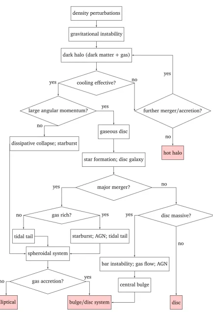
1.2 Logic flow chart for aΛCold Dark Matter model of galaxy formation . . . 3

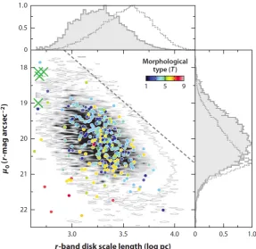
1.3 Distribution between the disc scale length and central surface brightness . . . 5

1.4 The evolution of the fraction of the different galaxy morphologies as a function of redshift from Mortlock et al. (2013). Further analysis has shown that there is a downsizing trend such that the most massive galaxies form into Hubble sequence galaxies earlier than lower mass galaxies Mortlock et al. (2013). . . 7

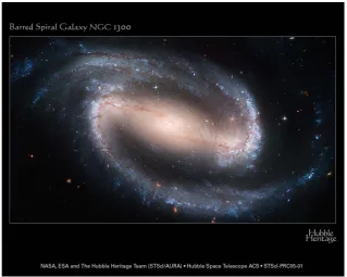
1.5 Barred spiral galaxy NGC 1300 . . . 10

1.6 Sombrero (M104) galaxy . . . 12

1.7 Original two-component fits from Kent (1985). . . 13

1.8 Spectroscopic measurements for two bulge-disc galaxies from MacArthur et al. (2008). Left panels: Color ACS images and slit orientations. Centre panels: Observed central galaxy spectrum (black lines) and the best fitting stellar template (red lines) con-volved to the measured velocity dispersion. Right panels: Kinematic profiles. Top: Velocity dispersion as a function of the light-weighted radius. Bottom: Radial veloc-ity profiles (i.e. rotation curves), shifted to zero velocveloc-ity at the centre. The vertical dashed lines indicate the effective radii for both the bulge and the disc. . . 17

1.9 Morphology diagram . . . 19

1.10 Image of NGC 4546, example of a boxy bulge . . . 20

1.11 Image of NGC 3370, example of a disc-like bulge . . . 21

2.1 The control flow of the 2D photometric decomposition MCMC algorithm. . . 32

2.2 A range of two-component models with the intensity along the y-axis and the radius normalised with the effective radius of the Sérsic profile on the x-axis. The black solid line is a Sérsic profile withn=1. Each frame has a different value of the ratioR_e/h with exponential component designated with the coloured lines. The colour of the line represents both theB/T shown in the larger colour bar on the right and theB/D within one effective radius shown by the individual colour bars to the right of each frame. . . 35

resents one parameter. The left column shows the Sérsic profile parameters; the ef-fective intensity,Ie, the effective radius,Re, and the Sérsic index,n. The right column

shows the exponential profile structural parameters; the central intensity,I0 and the

scale lengthh. The red, orange, green and blue corresponds to the 1st, the transition, the 2nd and the final level of the algorithm. The light blue segment represents the

burn-in which is discarded with only the final dark blue segment taken as a sample. . 42

2.5 Posterior marginals for a synthetic galaxy. The full marginal distribution for each of the structural parameters is shown on the diagonal. Joint marginal pairs of param-eters are shown on the off-diagonals. The seven color contours represent the 10, 30, 50, 68, 80, 95, and 99% confidence levels and the black solid line signifies 68% confidence level. The solid grey line shows the true value of this synthetic galaxy and the dashed line represents the median of the posterior distribution. There is a strong covariance between all the Sérsic profile parameters as well as the exponen-tial profile parameters. Although, evidence for a weaker covariance between the two components also exists. . . 48

3.1 Cosmological distance measures . . . 56

3.2 Spectral energy distributions . . . 60

3.3 Sesic profile . . . 62

3.4 Moffat profile . . . 65

3.5 CANDELS PDF . . . 66

3.6 Posterior error distribution for the entire ensemble of synthetic elliptical galaxies. The full marginal error distribution for each structural model parameter is shown on the diagonal. Joint marginal pairs of parameters are shown on the off-diagonal. The seven color contours represent the 10, 30, 50, 68, 80, 95, and 99% confidence levels and the black solid line signifies the 68% confidence level. The solid grey line shows the true value of this synthetic galaxy and the dashed line represents the median of the stacked posterior distribution. All the parameter values have some degree of correlation with the most correlated parameters being the Sérsic profile parameters between each other. . . 69

3.7 Posterior error distribution for the entire ensemble of synthetic bulge+disc galaxies. Lines and contours are the same as figure 3.6. . . 70

3.8 Box-plots representing the posterior errors of thenvs. binned true input values forI_e, Re,n,B/T, the ratio betweenRe and the PDF FWHM, and the ratio betweenReand h. The box limits represent the 16 and the 84% percentiles and the median values for each bin are shown in the horizontal line cutting each box. The whiskers show the extent of the distributions in each bin. . . 72

3.9 Same as Figure 3.8 but showing the posterior errors ofI_e,R_e,I0andhvs. binned true input values forn. . . 73

3.11 Same as Figure 3.8 but showing the posterior errors ofI0andhvs. binned true input

values forB/T,I₀andh. . . 76

3.12 Results from a MCMC decomposition for a galaxy from the SDSS sample. The top row shows the data (left), the Sérsic only model fit (middle) and the residual. The second row shows the exponential only fit and its corresponding residual. The bottom row shows the bulge-disc model fit and its corresponding residual. All the models were made using the medians from the posterior distributions. . . 77

3.13 Differences between parameter estimates for the elliptical galaxies where the model is a single Sérsic profile. From the top to bottom the parameters are: the effective intensity, I_e, the effective radius, R_e and the Sérsic index, n. Blue open circles are the posterior medians given by

PHI

PHI

PHI

PHI

3.14 Differences between parameter estimates for the disc+bulge galaxies where the model is a Sérsic profile plus an exponential. From top- to-bottom the parameters are: the effective intensity,Ie, the effective radius,Re, the Sérsic index,n, the central intensity

I0, and the scale length,h. See figure 3.13 for more details. . . 81

3.15 Ellipse-averaged surface brightness radial profile for an observed galaxy from SDSS (black dots) with the root mean square error from the pixel values in the image (grey region). The green band signifies model galaxies generated (and PSF convolved) from random draws from the output posterior distribution using a Sérsic and Sér-sic+exponential model ( left and right panels respectively). The blue band shows the random draws for the exponential component and the red band shows that for the Sérsic component without PSF convolution. The lower panel shows the residuals between the model (created with the posterior median) and the data. . . 83

3.16 Histograms (and cumulative distributions) showing the∆BIC distributions for syn-thetic single and two-component galaxies, the sample of SDSS galaxies classified by Gadotti (2009), and galaxies that are more likely to be single component according to the results from the machine learning approach by Huertas-Company et al 2011 (Top, middle and bottom panels respectively). As∆BIC=BIC_S´ersic−BIC_{S´ersic+e x ponent ial} a more positive value signifies the preferred model is that of two-components. . . 84

4.1 A succinct representation of a) a non-hierarchical model, whereDis the j thobserved data which is described by a set of parametersθ and b) a hierarchical model withD

andθtaking on the same meaning but nowθis described by a set of hyperparameters

φ. . . 89

jacent bins are anti-correlated as expected from the Dirichlet model, as adjacent bins will likely draw from similar galaxy posteriors. Dashed lines show the posterior me-dians for each fractional count parameter. . . 97

4.4 The global population used as a test case for the 2D Bayesian histogram. Each point has a full probability density function that is not shown. . . 99

4.5 The 2D Bayesian histogram representation of the test populationX and Y. The bin colours show the median proabability for the fractional count in each bin. The solid line shows the input model with the 1-sigma uncertainty added to the population shown by the dashed lines. . . 100

4.6 Figure showing the benefits of using the HBM. The top panel shows an example from the HBM of theRe−nplane for the two-component galaxies from SDSS (see Section

4.4.3). Refer to the colour bar in Fig. 4.5 for the bin values. The middle panel shows the 1, 2, and 3σcontours for the posterior distributions for the entire SDSS two-component population. The grey lines indicate the medians for the distributions. The bottom panel shows the full posterior probability distributions for a sub-sample from the two-component SDSS galaxies. . . 101

4.7 The top panel shows the cumulative distributions of the∆BIC values for the sample of SDSS galaxies split by their likelihood of being elliptical as derived by Huertas-Company et al 2011. As∆BIC increases the distance between the two distributions decreases with a minimum at∆BIC_≈25 (As∆BIC=BIC_S´ersic−BIC_{S´ersic+e x ponent ial} a more positive value signifies the preferred model is that of two-components). The red line shows galaxies that have a probability of being elliptical greater than 0.5 and the blue line shows the remaining galaxies. The next two panels show the results of a Kolmogorov-Smirnov test on the two distributions. . . 104

4.8 Results of the HBM for a sample of galaxies defined to be most likely single compo-nent system (∆BIC<25). The black histogram shows the results of the one dimen-sional HBM with error bars showing the 16% and 84% percentiles for the effective surface brightness. The blue histograms show the marginalised representation of the two dimensional HBM results betweenµ_eandR_e, whereas the red histogram shows the HBM results betweenµ_e and the Sérsic index, n. The bottom panels show the residuals between the 1DHBM and the 2DHBM in each case. . . 105

4.9 Similar to Fig. 4.8 but now showing the results of the 1DHBM (black histogram) and 2DHBM (blue histogram) for the effective radius (left) and the Sérsic index (right) for our one-component galaxies. . . 107

4.10 Results of the 1DHBM forµ_e,Re,n,µ0,hand the bulge-to-totalB/T(and disc-to-total D/T shown with the dashed line) ratio for the two-component galaxies in the sample. 109

4.11 The results from the 2DHBM for the Sérsic parameters for the one component galax-ies (left) and the two-component galaxgalax-ies (right). The first row showsµ_evs. R_e, the second row shows the KR or the mean effective surface brightness vs.R_eand the last row showsnversesRe. The colours for each bin represent the median posterior

prob-ability for the fraction of objects in that bin. A full posterior distribution is calculated for each bin, but not shown here. Refer to the colour bar in Fig. 4.5 for the bin values. 111

4.13 Similar to Fig.4.11 showing the bulge-to-total ratio for two-component galaxies plot-ted against the effective surface brightness,the effective radius and the Sérsic index. They all follow similar correlations with increasing log(B/T). . . 113 4.14 The results from the 2DHBM for the exponential profile parametersµ0 andh. . . 114

4.15 The left panel shows the results for the 2DHBM for the Sérsic parametersµ_e,Reand

nverses the disc sclae lengthh. The right panel shows again the Sérsic parameters

µeandnbut now verse the ratioRe/h. . . 116

4.16 The results of the 2DHBM for the Sérsic parameters of the elliptical galaxies (top row) and the disc galaxies (bottom row). The 1DHBM results fornare presented in the histograms with the error bars representing the 16% and the 84% percentiles as before. . . 117

5.1 Footprint of the CANDELS observations in the COSMOS field with WFC3/IR prime exposures shown in blue and ACS/WFC parallel exposures shown in magenta. (From Grogin et al. 2011) . . . 122

5.2 The mass evolution of galaxy populations is shown tracked from a redshift z = 2 to z = 0. The coloured bands are mass estimates from stellar population models combined according to a bulge-to-total ratio so that the result is matches a galaxy with logM_∗/M = 10 (left panel) and Milky-Way sized (logM_∗/M = 10.66; right panel) galaxy atz_∼0. The stellar populations are randomised for each component of the galaxy from: a single stellar burst model, an exponentially declining SFH and a constant SFH. The dashed line is the mass evolution function for a logM_∗/M=10.66 Milky-Way type galaxy from van Dokkum et al. (2013). The dashed-dotted lines are the mass evolution functions for galaxies with mass logM_∗/M =10.27, 11.2 from Ilbert et al (2013) and Patel et al (2013) respectively. The vertical dotted lines indicate the redshift ranges obtained from the morphological k-correction analysis described in the above text. . . 126

5.3 Stellar mass as a function of photometric redshift for the galaxies in the COSMOS field described in the catalogues of the 3D-HST project. The boxes indicate our cuts in mass and redshift according to the morphological k-correction of the SDSS i-band filter to the CANDELS WFC3/IR filters and the mass evolutions from the toy models. The blue boxes show galaxy masses that will evolve to become galaxies with masses logM_∗/M < 10.66 at z ∼ 0, and vice versa for the red boxes i.e. logM_∗/M >

10.66. The green boxes show galaxies that have the potential to evolve to become logM_∗/M = 10.66 or Milky-Way like masses. Mass ranges are all estimated from the toy models explained in the above text. For reference, the dashed line is the mass evolution function for a logM_∗/M=10.66 Milky-Way type galaxy from van Dokkum et al. (2013). . . 128

5.4 Results from the MCMC decompositions for three galaxies from the COSMOS sample. The images are placed in order of their corresponding∆BIC value. The top row has

∆BIC_≤ 0, the middle row has∆BIC_∼0, and the bottom row has∆BIC_≥ 0. The top row shows the data (left), the Sérsic only model fit (middle) and the residual. The second row shows the data (left), the bulge-disc model fit and its corresponding residual. The bottom row shows the bulge-disc model fit and its corresponding resid-ual. All the models were made using the medians from the posterior distributions.

for the three redshift ranges (median values for the redshift bins are shown) and two mass bins in the SDSS and COSMOS sample. The blue open circles show the lower mass samples (i.e, galaxies according to our toy models are likely to evolve to become log(M_∗/M)<10.66, blue boxes in Fig. 5.3) and the red closed circles show the higher mass sample (green and the red boxes in Fig. 5.3). The purple stars are the first two data points from Margalef-Bentabol et al. (2016) in their Figure 8 where all galaxies have a mass log(M_∗/M)_≥10.0. . . 132 5.6 The results from the 1DHBM for theR_eof the most probable single component

galax-ies. The top row shows results for the high mass sub-sample and the bottom row show the lower mass galaxy populations for the three redshift binsz∼0, 0.7 and 1 (left to right). The values of the histograms are the median values for the fractional counts for each bin estimated with the 1DHBM, and the error bars show the 16th and 84th percentiles. . . 133

5.7 Similar to Fig.5.6 but showing the results from the population distribution fornfrom the 1DHBM for the most probable single component galaxies. . . 134

5.8 Effective radius and Sérsic index as a function of redshift of the one component galax-ies, for our high mass sample (red filled circle) and low mass sample (blue circle) with the dashed lines showing the 1-σ error margins. We compare to the local elliptical sample from Gadotti (2009; grey open square), local massive (M_∗>1011M) galaxy sample from Szomoru et al. (2012; grey cross), Milky-way progenitor galaxies from van Dokkum et al. (2013; orange downward facing triangle) and M_∗ = 1011.2M

progenitor galaxies taken from Patel et al. (2013; line green right facing triangles). The grey box shows the PSF FWHM/2 limiting region over the high redshift range of our analysis. . . 137

5.9 Results from the 2DHBM of the Sérsic parameters for the one component galaxies defined by the∆BIC. From top to bottom: the effective surface brightness, the av-erage effective surface brightness (without cosmological surface brightness dimming corrections) and nvs. R_e within the difference redshift ranges. The contour levels describe the most likely regions defined by the medians for each bin described by the 2DHBM. The red contours are for the high mass sample and the black contours are for the low mass sample. The contours show the 1, 2, and 3σconfidence regions. . 138

5.10 Similar to Fig.5.9 but showing the results from the 2DHBMµ_e−nplane for the single component systems over the redshift range 0<z<1.27. . . 139

5.11 Probability contours for theRe−nplane from the 2DHBM for the single component

galaxies. The top row shows the high mass sample and the lower row are the lower mass objects. We show how the populations evolve fromz_∼1 toz_∼0.7 andz_∼0.7 toz∼0. In each panel, the red dashed contours compares how the population at the higher redshift bin is to the immediate lower redshift bin (black solid contours). . . 140

5.13 Similar to Fig.5.12 but showing the results from the population distribution fornfrom the 1DHBM for the most probable two-component galaxies. . . 142

5.14 Effective radius and Sérsic index as a function of redshift of the two-component galax-ies, for our high mass sample (red filled circle) and low mass sample (blue circle) with the dashed lines showing the 1-σerror margins. We compare to the local sam-ple from Gadotti (2009; pseudo-bulges is the grey open square and classical bulges is the closed grey square). The cyan open diamonds and dark red closed diamonds show the pseudo and classical bulges from Sachdeva, Saha and Sihgh (2017) respec-tively. The purple left-facing triangles show the results from Margalef-Bentabol et al. (2016) for the bulges of there two-component galaxies. The grey box shows the PSF FWHM/2 limiting region over the high redshift range of our analysis. . . 143

5.15 The 2DHBM of the Sérsic parameters for the two-component galaxies defined by the

∆BIC. From top to bottom: the effective surface brightness, the average surface brightness andn versesR_e within the different redshift ranges. The contour levels describe the most likely regions defined by the medians for each bin described by the 2DHBM. The red contours are for the high mass sample and the black contours are for the low mass sample. . . 145

5.16 Similar to Fig.5.11 showing the probability contours for theRe−nplane from the

2DHBM for the two-component galaxies. The top row shows the high mass sample and the lower row are the lower mass objects. We show how the populations evolve fromz∼1 toz∼0.7 andz ∼0.7 to z∼0. In each panel, the red dashed contours compares how the population at the higher redshift bin is to the immediate lower redshift bin (black solid contours). . . 146

5.17 Similar to Fig.5.12 showing the results from the 1DHBM for theB/T probability dis-tribution of the two-component galaxies. . . 147

5.18 Probability of the high mass (filled circle-dashed line) and low mass (circle-solid line) populations according to theirB/T values (indicated by the colour code in the upper right legend) as a function ofz. Also shown is the number fractions from the study by Bruce et al. (2012) for galaxies with M_∗ > 1011M (triangle-dashed line). The open squares indicate the full sample from Gadotti (2009) and the half-circles show the results from Fisher & Drory 2011 (M_∗ > 109M). The filled regions indicated the number fraction of the semi-empirical galaxies more massive than 1011M from Avila-Reese et al. 2014. The contrasting mass rages make direct comparisons diffi-cult, although the trends do indicate the importance of mass in galaxy evolutionary scenarios. . . 148

5.19 Similar to Fig.5.16 but showing the probability contours for theB/T₋R_eplane from the 2DHBM for the two-component galaxies. . . 150

5.20 Similar to Fig.5.16 but showing the probability contours for theB/T₋nplane from the 2DHBM for the two-component galaxies. . . 151

5.21 Similar to Fig.5.12 showing the results from the 1DHBM for thehprobability distri-bution of the two-component galaxies. . . 153

eters from the 2DHBM for the two-component galaxies. . . 154

5.24 Similar to Fig.5.16 but showing the probability contours ofB/Tverses the exponential parameters from the 2DHBM for the two-component galaxies. The red and black contours are for the high mass and low mass populations respectively. . . 155

5.25 Similar to Fig.5.16 but showing the probability contours of the ratio betweenR_eand

hversesnfrom the 2DHBM for the two-component galaxies. . . 156

5.26 A schematic of the evolution for the one-component galaxies sincez∼1. The arrows show the overall growth of the galaxies shown by the results earlier in this chapter. The compact progenitors (red box) may take one of two paths: (1) either they grow rapidly due to dry minor mergers which deposit material onto their outer parts (lead-ing to the local high mass one-component scal(lead-ing relation shown by the red ellipse) or (2) infalling gas forms a disc around the spheroid becomingz_∼0 bulge-dominated two-component galaxies. The high mass, extended, one-component galaxies atz∼1 could become the discs of the modern disc-dominated galaxies and most likely form a bulge (blue box). Whereas evidence suggests that the lower mass extended galaxies atz ∼1 could become the population of modern pure disc galaxies. However, this may be dependent of the enviroment around the galaxy. . . 161

List of Tables

2.1 Input parameters and priors used in the MCMC code. . . 40

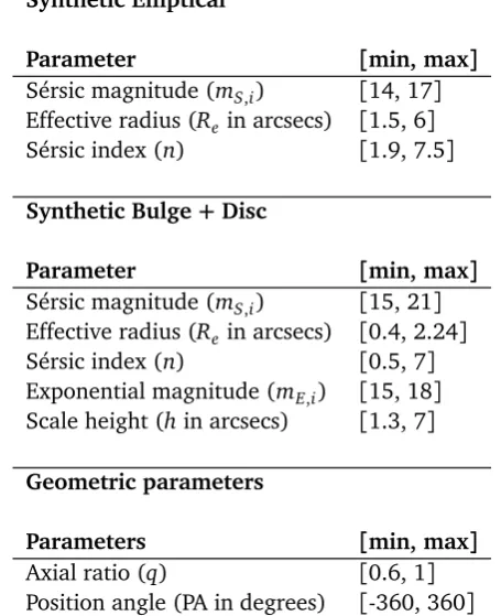
3.1 Parameter ranges for synthetic single component Sérsic galaxies and two-component Sérsic+Exponential galaxies. Geometric parameter ranges are also shown. . . 67

3.2 Table showing the medians of the posterior errors shown in Figures 3.6 and 3.7 along with the 16th and 84th percentiles for the synthetic elliptical and bulge+disc galaxies. 68

3.3 Table showing the statistics for Figure 3.16 of the∆BIC distributions in the synthetic and SDSS samples. . . 85

4.1 Summary of our notation . . . 91

4.2 Statistics for the distributions derived from the 1DHBM for each of the population parameters. . . 108

5.1 Table containing the number of galaxies in each redshift and mass bin . . . 129

5.2 Results for the one-component galaxies. . . 135

1

Introduction

1.1

Historical concepts of galaxies

Lost somewhere between immensity and eternity, is where Sagan (1981) placed us in the opening

chapters of the supporting material to his award-winning television series, ‘Cosmos: A Personal

Voyage’. The Milky Way was believed to occupy more or less the whole Universe at the beginning

of the twentieth century. The idea that extragalactic systems could exist was not established until

the 1920’s, with the pioneering efforts from some of the most renowned astronomers. The name

nebulae was given to these fuzzy objects that clearly were not stars. Edwin Hubble proved that

these objects were indeed other galaxies, much like our own, external to our island of stars, some at

colossal distances from us. Hubble (1926) first classified these galaxies according to their apparent

morphology into what is now known as the Hubble tuning fork (Figure 1.1). This classification is still

present today, and is used to break the population of galaxies down into eitherelliptical,lenticular,

spiralorirregularclassifications, with the existence of extra features such as bars, dividing objects

into subclasses. The different classifications are a reflection of the different properties and forms

Figure 1.1: The original schematic of Hubble’s tuning fork as published in 1936 in his Realm of the Nebulae. The elliptical galaxies are presented on the left hand side ranging from E0 - E6, with lenticular galaxies presented as S0. The right hand side shows the spiral galaxies split by the presence of a bar.

understand the physical mechanisms that shape them.

1.2

Galaxy formation: From nothing to something

The following section is an overview of the basic theoretical framework of our current model of how

structure forms in the Universe, a logic flow chart is presented (see Figure 1.2) to guide the reader

and to highlight the main focus of this thesis.

Galaxy formation models currently favour a cold dark matter cosmology (Blumenthal et al.,

1984). The cosmic microwave background is explained successfully with this model (Komatsu et al.,

2009), furthermore, there is substantial evidence that the model describes the observed large scale

structure of the Universe (Benson, 2010 and references therein).

Structures in the Universe are thought to come about through minute matter density

fluctua-tions, expanded to cosmological scales by inflation (Liddle, 1999). As the dark matter component is

entirely governed by gravitational forces, denser regions will collapse, increasing the perturbations.

The linear theory of cosmological perturbations provides an accurate description of the early

evo-lution of these perturbations (Shaw & Mota, 2008). Once the perturbation reaches some threshold

over-density, it breaks away from the expansion and begins to collapse. This transition signifies

non-linear perturbations (Shaw & Mota, 2008).

The consequence of the non-linear, gravitational collapse depends on the denser regions of dark

matter and baryonic matter. An approximately stable, near-equilibrium state supported against its

1.2. Galaxy formation: From nothing to something

density perturbations

gravitational instability

dark halo (dark matter+gas)

cooling effective?

large angular momentum? further merger/accretion?

hot halo gaseous disc

dissipative collapse; starburst

star formation; disc galaxy

major merger?

disc massive? gas rich?

bar instability; gas flow; AGN

central bulge starburst; AGN; tidal tail

tidal tail

spheroidal system

gas accretion?

elliptical bulge/disc system disc

yes

yes

no no

no

yes

no yes

no yes yes

no

no yes

own self-gravity is the result of this nonlinear evolution of the dark matter density perturbation,

known as the dark matter halo. Halo density profiles, shapes, spins and, internal substructure all

depend weakly on either mass or cosmology, although the abundance and characteristic density is

finely dependent on these (e.g.,Eke et al. 1996).

Initially, baryons are thought to be uniformly distributed, tracing the dark matter distribution on

scales above the Jeans length (Gnedin & Hui, 1998). Dark matter potential wells are expected to

concentrate the force of gravity creating galaxy formation sites. Both the depth of the potential well

and the pressure of the baryons will determine how much is accreted into the structure. The cooling

of the gas is a vital ingredient to galaxy formation. The overall effect of cooling segregates the

baryonic material from the dark matter, and it accumulates as dense, cold gas in the protogalaxy,

situated in the centre of the halo. The nature of the cooling process is largely dependent on the

atomic species of the gas (different excitation energies) and the initial density. For more insight into

cooling with a specific focus into different properties/mechanisms, see the review by Benson (2010)

and references therein.

The collapse of baryonic matter is reliant on it being cool, however, this process also leads to the

heating of the gas; increased density and temperature leads to the extension of the cooling time.

During the collapse the gas may fragment into clumps of small, highly dense cores, finally resulting

in the formation of stars. Star formation theory is a broad field in itself and much time and effort

has been spent on understanding it (see the review by McKee & Ostriker 2007).

The original concept given to galaxies was theislanduniverse. In some cases this can be a

rea-sonable assumption, whereby the galaxy spends most of its time in isolation. Although, in recent

decades, evidence of merging galaxies have been observed. The merging together of less massive

dark matter halos appears to be the hierarchical nature of structure formation in the Universe, with

current high resolution simulations supporting this (Kuhlen et al., 2008). There has also been

con-siderable work in the hierarchical build up of merger trees, which can be thought of as the back-bone

to galaxy formation (Jiang & van den Bosch 2014, also see Mo et al. 2010 for more details on the

theory behind mergers).

Through the gravitational influence from the dark matter halos, the gas will now have a

suffi-ciently high density to allow a galaxy to form. The shape that the galaxy will have will depend highly

on its composition and the properties of its components (e.g.,gas and dark matter). To characterise

this branch in the galactic evolution tree which involves the internal dynamical effects, the tidal

1.3. The Stellar Disc

the reader will soon find out, this thesis can reside within this field of research. But how do we go

from a dense gas cloud within the potential well of a dark matter halo to the galaxies we see today?

The following sections will describe in detail the formation of discs, galactic bulges and the various

sub-structures within.

1.3

The Stellar Disc

Disc galaxies in general consist of a disc component made up of stars, dust, cold gas (atomic and

molecular), a central bulge (discussed more in Section 1.4), a stellar halo, and a dark matter halo.

The discs sometimes have very distinctive features such as spiral arms and/or bar components (see

Section 1.3.4). A theoretical framework for the galactic disc needs to account for these specific

features as well as a variety of observational facts.

1.3.1

Observational properties

Observations of disc galaxies show that on average, smaller discs have higher surface brightnesses.

One of the most fundamental parameters describing the morphology of disc galaxies is the scale

length (h). It describes how the stars within the disc are distributed. Assuming a specific

mass-to-light ratio, the scale length can also be used to derive the mass distribution (Fathi et al., 2010). Figure

1.3 taken from Fathi (2010) (adapted in van der Kruit & Freeman 2011) shows the relation between

the central surface brightness (µ₀) and the scale length of the disc, suggesting a link between the

size of the disc and its brightness.

The radial distribution of surface brightness distribution in the discs of face-on or slightly inclined

galaxies can be approximated to be an exponential of the form,

I(R) =I₀exp(₋R/h) (1.1) whereI(R)is the intensity as a function of radius,R, in the disc with a central intensityI0 and scale

length,h. Freeman (1970) was the original publication suggesting exponential discs, where B-band

observations were used. Freeman (1970) also identified that discs can sometimes differ from the

simple exponential profile.

Disc profiles were classified into two groups: type I discs had the simple exponential form,

while, type II discs show an outer exponential fall-off, with the inner part sometimes falling below

the inward projection of the outer exponential (Freeman, 1970). Type II discs can be identified

from the truncation of the stellar population at large radii, roughly 2-4 scale lengths (van der Kruit

& Searle, 1981b,a; Pohlen et al., 2002). Using images from face-on galaxies, Pohlen et al. (2002)

was able to show that the truncation changes from the shallow exponential of the main disc to the

steeper exponential at larger radii. Thus, truncations can be identified as another form of Freeman’s

type II disc profiles. More recent work, shown through radial surface brightness profiles of

early-type galaxies (Erwin et al., 2005) and late-early-type discs (Pohlen & Trujillo, 2006) presents evidence

for a third type of profile. Erwin et al. (2005) classify this type III disc profile as ‘anti-truncation’:

the outer profiles are distinctly shallower in slope than the main disk profile. For a more detailed

analysis of galaxy disc properties see the review by van der Kruit & Freeman (2011).

Brighter discs tend to be of a redder colour, although observations show significant scatter. de

1.3. The Stellar Disc

bluer colours. The results come about from the mean stellar ages and metallicity and not from

the absorption by dust. The work presented in de Jong (1996) show disc galaxies having colour

gradients, with the outer regions being bluer than the inner regions.

Another observational quality of bright disc galaxies is that they will be fast rotators ( high

circular-speed). Discs tend to have flat rotation curves. The circular velocity of massive galaxies

tends to rise rapidly at small radii then is almost constant thereafter (Begeman, 1989). Swaters

et al. (2000) presented high-resolution Hα rotation curves of LSB galaxies, which were found to

have a flat curve out beyond two scale lengths similar to the massive galaxies. The rotation is a

direct measure of the gravitational force within the disc, and can be used as a trace of dark matter.

The rotation rate of the spirals in the flat part of the circular-speed curve is related to the luminosity

of the host galaxies, this is known as the Tully-Fisher relation (L ∝ v_c3.5) (Tully & Fisher, 1987). The rotation can be measured using a range of techniques, the most common being optical long slit

or IFU spectroscopy of HII region emission lines.

1.3.2

High redshift disc observations

Figure 1.4: The evolution of the fraction of the different galaxy morphologies as a function of redshift from Mortlock et al. (2013). Further analysis has shown that there is a downsizing trend such that the most massive galaxies form into Hubble sequence galaxies earlier than lower mass galaxies Mortlock et al. (2013).

With the advent of the Hubble Deep Fields (HDF) (Williams et al. 1996; Ferguson et al. 2001),

the field of high redshift studies has changed drastically since the late 90’s. The HDF, and later very

deep imaging campaigns, such as the Hubble Deep Field South (Williams et al. 2000), the Great

Observatories Origins Deep Survey (GOODS) (Giavalisco et al. 2004), the Hubble Ultra Deep Field

(UDF) (Beckwith et al. 2006), the COSMOS field (Scoville et al. 2004), the Extended Growth Strip

2011), have revolutionised the field of galaxy formation and evolution studies, in particular to the

study of morphologies.

The critical nature of these deep fields was to obtain photometry at the faintest levels possible in

a wide range of bands. Usingphotometric redshiftestimation methods (see Dahlem et al. (2013) for

a discussion on this method), redshifts for distant galaxies were obtained. These redshifts allowed

astronomers to study the evolution over a broad redshift range which was not possible before.

Figure 1.4 shows the evolution of visual morphologies, as defined solely by visual types, from

Mortlock et al. (2013) for systems with stellar masses M_∗ >1010M. The classification of a

spi-ral, elliptical or peculiar/irregular does not imply that these galaxies have certain properties only

that they are visually the same as these classes, as defined in the local Universe. What Figure 1.4

shows is that at z > 2 the dominant morphological type is peculiar, while the elliptical and disc

galaxies become more populous at lower redshifts (also see Conselice et al. 2005; Kriek et al. 2009;

Delgado-Serrano et al. 2010; Mortlock et al. 2013). The Universe is not dominated by the types of

morphologies seen in the local Universe untilz_∼1.9 (Mortlock et al. 2013). However, galaxies that

share similar physical properties with type - such as colours, star forming knots, and tidal features,

have not reached the same level as local galaxies at this redshift (Conselice 2014).

How galaxies evolve needs to be addressed with the use of parametric and non-parametric

meth-ods. One quantitative measure to observe the evolution of galaxy structures is through the evolution

of the Sérsic index,n(Sersic, 1968). The Sérsic model will be discussed in more depth in Chapter 2

but generallynis commonly linked to the shape of a galaxy. Lowernvalues are associated to more

discyobjects whereas highernvalues are connected with more concentrated galaxy structures such

as ellipticals. Previous studies of the evolution of derived values ofnas a function of redshift show

that galaxies have lowernvalues at higher redshift (e.g. Buitrago et al. 2013). Some studies have

implied that these galaxies are more disc-like at high redshifts (Bruce et al. 2012), although

com-parisons to the visual inspection of these systems as well as their physical properties, find they are

dissimilar to discs in the local Universe (Conselice et al. 2011; Mortlock et al. 2013). Although these

disc-like galaxies have similar light profiles to modern discs they have been observed to be much

smaller, have higher stellar masses, and are often undergoing intense star formation making them

un-disc-like in regards to the discs observed in the nearby Universe (Shen et al. 2003; Conselice et

al. 2011; Buitrago et al. 2013). The question still remains as to how these progenitor galaxies help

1.3. The Stellar Disc

1.3.3

The origins of the exponential disc

The origin of the exponential stellar disc still remains a challenge in disc formation models. Freeman

(1970) specified that the distribution of angular momentum in a self-gravitating exponential disc

closely resembles that of a uniformly rotating, uniform sphere. An exponential density distribution

with a flat rotation curve also shows similarities (Gunn, 1982; van der Kruit, 1987). To approach

this problem, two concepts have been considered; (a) essentially what Freeman (1970) suggested

with the surface density distribution of the disc galaxy reflecting the specific angular momentum

dis-tribution of the proto-galaxy and (b) the surface density disdis-tribution is a result of disc viscosity (Lin

& Pringle 1987). Unfortunately both approaches still have their problems. Yoshii & Sommer-Larsen

(1989) made an early attempt to describe the formation of the exponential profile. It was shown

that an exponential disc could form if the time scales for viscosity and the formation of stars was

comparable (also see Slyz et al. 2002 where hydrodynamical simulations of disc galaxies were used

to shed new light on the formation and evolution of disc galaxies). It has also been suggested that a

disc model with a detailed conservation of angular momentum would give a natural explanation for

the exponential profile, potentially forming the truncations as well (Fall & Efstathiou, 1980).

How-ever, other non-antisymmetric structures such as bars may redistribute angular momentum, thus

it is important to characterise the main properties of these non-axisymmetric structurese.g., spiral

arms (Debattista, 2006), in order to shed light on the formation and evolution of discs.

1.3.4

Bars & spiral arms

Stellar bars are quasi-elliptical structures (see Figure 1.5 for an example barred galaxy) which are

present in approximately two-thirds of all spiral galaxies in the local Universe (Marinova & Jogee

2007; Menéndez-Delmestre et al. 2007; Aguerri, Méndez-Abreu et al. 2009). Early studies found

that the bar fraction evolves significantly (Abraham et al. 1999), while later studies find that bars

are already in place byz∼1 (Elmegreen, Elmegreen & Hirst 2004; Jogee et al. 2004; Marinova &

Jogee 2007). It was later shown that the bar fraction increases fromz=0.84 toz=0.2, from 20% to_∼60% of all disc galaxies (Sheth et al., 2008). Sheth et al. (2008) also find that the bar fraction

is roughly constant for the most massive and red disc galaxies with lower mass bluer discs showing

the most significant evolution.

In many barred spirals, the spiral arms appear to start at the two ends of the bar suggesting

that they are tightly related. It is now largely accepted that spiral structures seen in disc galaxies are

Figure 1.5: The barred spiral galaxy NGC 1300. NGC 1300 has been classified as a SBbc galaxy due to itsgrand-designspiral structure. [NASA and The Hubble Heritage Team (STScI/AURA)]

detail by Bertin & Lin 1996). These density waves can have a great impact on the stellar populations

within the galactic components. Numerical simulations show that a significant fraction of stars in

galaxy discs undergo large migrations in radius due to resonant scattering from the spiral arms

(Roškar et al., 2008a,b). Stars that are initially on circular orbits in the disc, will be scattered into

approximately circular orbits with larger radii if they lie near the co-rotation resonance (Roškar

et al., 2008b). This can lead to the formation of a steeper exponential decline in the outer disc

formed mainly from stars initially located in the central regions of the disc. It is suggested that this

process could smooth out the metallicity and age gradients, resulting in a galaxy with older, less

metal rich stars at the centre (Roškar et al., 2008b).

Numerical simulations show that the encounter of a disc galaxy with another galaxy can

pro-duce a bar-like structure in an otherwise stable disc (Noguchi, 1987). With the disruption of the

disc by the bar, a boxy/peanut bulge or a discy bulge may form (Athanassoula, 2008). This is a

pos-sible formation scenario for the disc-like bulge (or pseudo-bulge) outlined in Kormendy & Kennicutt

(2004). A disc-like bulge is one formed through secular processes in the disc rather than the result

1.4. Galactic Bulges

1.4

Galactic Bulges

The formation of the bulge component is key when modelling galaxy formation. But what is the

galactic bulge? The original meaning comes from the Latin word bulgawhich came to describe

the shape of a full bag. The modern Oxford dictionary defines it as a distortion in an otherwise flat

surface. Some authors follow this idea and define the bulge as the component that swells out of a disc

galaxy when viewed side-on (Figure 1.6 is an image of the Sombrero galaxy, a spiral galaxy seen edge

on with a prominent bulge). An early working definition comes from the Carnegie Atlas of Galaxies

(Sandage & Bedke, 1994); it states that one of the classification criteria for spiral galaxies is the size

of the central amorphous bulge compared to its disc, seen best in nearly edge-on galaxies. Carollo

et al. (1999) questions this definition finally concluding that of course bulges are an excess of light

(a higher surface brightness) than the inner disc. Another definition follows a more morphological

form. Renzini (1999) defines the bulge using the canonical interpretation of the Hubble-Sandage-de

Vaucouleurs classificationi.e., looking at bulges as ellipticals which have a prominent disc around

them, and vice versa for ellipticals that have not maintained a disc during their evolutionary path.

Thus defining what a bulge is is no easy task and the nomenclature has changed over the years.

With the advent of methods such as photometric decompositions, a more quantitative description

was adopted where the excess light that protrudes from an exponential disc quantifying the bulge

(Freeman 1970). This photometric definition of a bulge is widely used, usually modelled with

a Sérsic profile (Sersic, 1968) separating it from other structures such as discs and bars in

multi-component structure modelling (Gadotti 2009; Laurikainen et al. 2010; Méndez-Abreu et al. 2014).

Throughout this thesis we use this photometric description of galaxy bulges.

As observations improve, more features are being discovered which make it hard to distinguish

the bulge in this way. This leads to astronomers to ask whether bulges of early-type and late-type

spirals are really different? Can bulges of different types of galaxies be classified together? (Fathi

& Peletier, 2003). Thus, the most operative definition will be to consider the bulge as the extra

light in the central region above that of the inner disc. Readers should also recognise limitations in

this definition; is it even sensible to consider everything that is in excess of the inner disc to be the

bulge? Should we consider the nuclear components of the disc? For the present thesis, it will be

sufficient to proceed considering representative properties, leaving details aside until a higher level

Figure 1.6: Sombrero (M104) galaxy. A Sa galaxy hosting a central bulge[NASA and The Hubble Heritage Team (STScI/AURA)]

1.4.1

Observational properties

The advance of optical (CCD) and near-infra-red instruments in the late-80s and 90s meant that

full 2D data modelling was achievable which subsequently lead to a quick increase in the quality of

bulge photometry. Reliable photometric models for the bulge were then subtracted to understand

individual components of galaxies. The general features of bulges can now be described in a variety

of ways.

•Photometry: A morphological point of view

de Vaucouleurs (1948) produced the quantitative description of elliptical galaxies which was

ex-panded to bulges of disc galaxies, including the surface brightness profiles following the radius as

r1/4. Sersic (1968) improved this relation by replacing the 1/4 in the r1/4 law with 1/n, where

n is fitted to the data. Kent (1985) measured the shapes of bulges as well as their radial profiles

and concluded that the ellipticity shows little correlation with the effective surface brightness of

the bulge (see Figure 1.7). Kent (1985) stated that if all the bulges followed the same law, i.e.,

they were all oblate spheroids viewed from different directions, more edge on galaxies would have

a larger ellipticity thus they would have a higher surface brightness. The absence of this

corre-lation suggested that bulges must have more complex shapes than simple oblate spheroids. This

has been later confirmed due to the triaxiality of bulges (Méndez-Abreu et al., 2010). Andredakis

1.4. Galactic Bulges

Figure 1.7: two-component model fits to the observed profiles of two S0 galaxies from Kent (1985) were some of the first photometric fits to bulges were done. The solid line is the sum of the bulge and the disc with bulge and the disc components being represented by the short-dashed and the long-dashed lines respectively.

decomposition method for extracting K-band light profiles, fitting with the more general Sèrsic

pro-file, found early-type galaxies were better fit with a de Vaucouleurs profile while bulges in late type

galaxies had more of an exponential profile.

The r1/4 law was still used in bulge-disc decompositions as it was favoured for high redshift

(Simard et al., 2002) and early-type bulges. It was during this time that the use of the Sèrsic

pro-file began to seem more and more relevant in bulge-disc decompositions. Several studies including

early-type bulges (Khosroshahi et al., 2000; Graham, 2001) found that the bulge luminosity scaled

with the Sèrsic shape indices (from n<1 to n> 4). The central regions of the profile dominate

at higher values of the Sèrsic index. Bringing together knowledge of the inner regions of the disc

(Phillips et al., 1996), compact sources (Rest et al., 2001; Pizzella et al., 2002), and star formation

(Carollo et al., 2002), present in the galaxy centres, we begin to understand the difficulty in

disen-tangling the different light profiles. The sources present in the central regions contribute to the light

resulting in a highern value. For example, Balcells et al. (2003) used theHubble Space Telescope

(HST) near-infrared imaging instruments, to measure the surface brightness profiles of spiral

(S0-Sbc) galaxies at high resolution. The result found that nuclear point sources were blending with

the light of the bulge due to the point-source properties, namely the point spread function (PSF)

(Balcells et al., 2003).

•Kinematics

The study of motions of stars in galaxies reveals a wealth of dynamical information about these

determine the distribution of the stellar component within. Also obscuration due to dust further

complicates the analytical process as well as the mixing of stars making it a complex process in

separating different stellar components. Only line-of-sight velocities and angular coordinates are

observable. Until the seminal work of Kormendy & Illingworth (1982), astronomers held the

tra-ditional picture of bulges being elliptical galaxies with a disc. This idea was motivated by the very

similar properties observed for bulges and ellipticals, i.e., morphologies, stellar content, and the

re-lation between the luminosity and the central velocity dispersion (also known as the Faber-Jackson

relation, Faber & Jackson 1976). However, the bulges for which kinematics were available were all

situated in early-type spirals with large central regions. Kormendy & Illingworth (1982) studied the

relation between the ratio of the rotation velocity,V, and random motions,i.e,velocity dispersion,σ,

with the ellipticity,ε, of the galaxy. Evidence was provided that bulges follow the oblate-spheroid

picture. Kormendy (1982) then added to the previous list of intermediate wound spiral (S0-Sb)

bulges with a set of lens-shaped barred spirals (SB0) bulges. All the SB bulges were found to be

rotating at least as rapidly as the oblate-spheroids, with some rotating faster than previous estimates

for an isotropic rotator. This suggested that these systems contained more disc-like kinematics than

spheroidal.

The study of stellar kinematics took a giant leap with the discovery of thin, rotating discs

domi-nating the light in the inner parts of some galaxies, accompanied by a local minimum in the velocity

dispersion (Emsellem, 1998). Long slit spectroscopic observations of spiral galaxies show stellar

velocity dispersions (in the radial direction) were decreasing exponentially with radius (Bottema,

1989, 1993). With the integral-field spectrograph SAURON operating on the William Herschel

Tele-scope, Falcón-Barroso et al. (2006) was able to characterise the central local minima in the velocity

dispersions in some 13 Sa and Sab galaxies. The star formation rates (SFRs) in the sample were

similar to what was seen in normal disc galaxies, with the low velocity dispersions being linked to

regions of star formation. Evolution of the galaxy over a period of time similar to the dynamical

time of the galaxy could result in this velocity dispersion drop due to gas falling into the centres;

this process is discussed further in Section 1.4.3 on the formation theories of bulges.

•Stellar populations

Early population synthesis studies were performed with libraries of stellar spectra or libraries

con-taining stars and globular clusters. It wasn’t until Bica (1988) used a base of star cluster integrated

spectra to undertake a two parameter analysis composed of age and metallicity. From the age and

1.4. Galactic Bulges

Following the pioneering effort of Bica (1988), it soon became apparent that a

metallicity-luminosity (Z/L) relation was present (Jablonka et al., 1996; Idiart et al., 1996). Spectroscopic studies in the late nineties provided evidence for similarities in the metallicities of both spiral and

elliptical galaxies (Jablonka et al., 1996; Idiart et al., 1996). Similarities were held in the mean

metallicity, with ellipticals observed to have an Iron to Hydrogen ratio being roughly half that of

bulges. On the other hand, the αelements to Iron ratio, [α/Fe], was approximately equal to one

another. The stellar populations were suggested to scale with the central velocity dispersion and the

bulge luminosity rather than the classification of the galaxy (Jablonka et al., 1996). Comparisons

were later made between M31 and the Galactic bulge (Jablonka et al., 1998). 19 globular

clus-ters present in the central regions were found to be mostly metal-poor which was proclaimed to be

similar to the Galactic bulge. However, two of the 19 clusters observed were highly metal-rich and

compared well with the nuclei of giant ellipticals and the semi-stellar nucleus of M31 itself, these

metal-rich clusters in the core were deemed rare. Hammer et al. (2001) speculated that luminous

compact galaxies (LCGs) were instead the progenitors of bulges of massive spirals. Spectroscopic

observations of a sample of LCGs were compared to present day bulges of massive spirals.

Simi-larities were found in their stellar masses, metal abundances, along with evidence to suggest low

surface brightness components around the high surface brightness cores. While similarities maybe

present, the statement that LCGs are the progenitors to modern day bulges is a speculation (more

on the evolution scenarios will be discussed in Section 1.4.3).

Photometric studies of bulges situated in early-type galaxies show that they differ from bulges in

late-type spirals (Falcón-Barroso et al., 2002). Using HST, Falcón-Barroso et al. (2002) has showed

that bulges of later morphological types have slightly younger ages. The analysis of stellar

popula-tions through spectroscopic observapopula-tions of edge-on spiral galaxies spanning the Hubble sequence

show the vast majority of bulges are of an older age, lower metallicity and higher [α/Fe] in the

outer region than the central parts (Gorgas et al., 2007; Jablonka et al., 2007). Jablonka et al.

(2007) suggest that the effective radii and the Hubble type of the parent galaxies play a minor role

in causing spatial variations in the stellar populations.

1.4.2

High redshift bulges

Studying the high-redshift progenitors to local galaxies can provide us with invaluable insights into

the key mechanisms that drive the evolution of these galaxies, constraining parameters for the use

in formation models. Data from local galaxies cannot distinguish between the various evolutionary