Galaxy And Mass Assembly (GAMA) : stellar mass functions by Hubble type

Galaxy And Mass Assembly (GAMA): stellar mass functions

by Hubble type

Lee S. Kelvin,

Simon P. Driver,

Aaron S. G. Robotham,

Edward N. Taylor,

Alister W. Graham,

Mehmet Alpaslan,

Ivan Baldry,

Steven P. Bamford,

Amanda E. Bauer,

Joss Bland-Hawthorn,

Michael J. I. Brown,

Matthew Colless,

Christopher J. Conselice,

Benne W. Holwerda,

Andrew M. Hopkins,

Maritza A. Lara-L´opez,

Jochen Liske,

Angel R. L´opez-S´anchez,

´

Jon Loveday,

Peder Norberg,

Steven Phillipps,

Cristina C. Popescu,

Matthew Prescott,

Anne E. Sansom

and Richard J. Tuffs

Accepted 2014 July 24. Received 2014 July 4; in original form 2013 November 11

A B S T R A C T

We present an estimate of the galaxy stellar mass function and its division by morphological type in the local (0.025< z <0.06) Universe. Adopting robust morphological classifications as previously presented (Kelvin et al.) for a sample of 3727 galaxies taken from the Galaxy And Mass Assembly survey, we define a local volume and stellar mass limited sub-sample of 2711 galaxies to a lower stellar mass limit ofM=109.0M. We confirm that the galaxy stellar mass function is well described by a double-Schechter function given byM∗=1010.64_M

,

α1 = −0.43,φ∗1 =4.18 dex−1Mpc−3,α2 = −1.50 andφ∗2 =0.74 dex−1Mpc−3. The

con-stituent morphological-type stellar mass functions are well sampled above our lower stellar mass limit, excepting the faint little blue spheroid population of galaxies. We find approx-imately 71+₋3₄ per cent of the stellar mass in the local Universe is found within spheroid-dominated galaxies; ellipticals and S0-Sas. The remaining 29+₋4₃per cent falls predominantly within late-type disc-dominated systems, Sab-Scds and Sd-Irrs. Adopting reasonable bulge-to-total ratios implies that approximately half the stellar mass today resides in spheroidal structures, and half in disc structures. Within this local sample, we find approximate stellar mass proportions for E : S0-Sa : Sab-Scd : Sd-Irr of 34 : 37 : 24 : 5.

Key words: galaxies: elliptical and lenticular, cD – galaxies: fundamental parameters – galaxies: luminosity function, mass function – galaxies: spiral.

1 I N T R O D U C T I O N

Amongst the veritable cornucopia of observed and derived galaxy parameters, the total stellar mass of a system is arguably one of the most fundamental, perhaps in conjunction with the shape of the galaxy light profile as parametrized by, e.g. the S´ersic (1963) func-tion. One common viewpoint has it that galaxies form via a series of monolithic collapse and/or hierarchical merging events, where-after evolution continues to occur via additional merging events and stochastic gas accretion phases (e.g. Navarro & Benz1991;

E-mail:[email protected]

White & Frenk1991; Wyse, Gilmore & Franx1997; Kereˇs et al. 2005; Debattista et al.2006; Khochfar & Silk2006a,b; De Lucia & Blaizot2007; Cook, Lapi & Granato2009; Cook et al.2010; van Dokkum et al.2010; Pichon et al.2011; Kormendy & Ben-der2012; L’Huillier, Combes & Semelin2012). Each stage during this galactic ageing process has an observational impact upon the instantaneous state of a galaxy, e.g. colour (Baldry et al. 2004; Baldry, Glazebrook & Driver2008), star formation rate (Behroozi, Wechsler & Conroy2013; Moustakas et al.2013), in addition to leaving a longer term imprint on the nature of the galaxy, e.g. metal-licity (De Lucia, Kauffmann & White2004; Driver et al.2013; Lara-L´opez et al.2013), structure (Cooper et al.2012; Robotham et al. 2013; Shankar et al.2013; Szomoru et al.2013). In many ways this

C

2014 The Authors

at University of St Andrews on December 8, 2014

http://mnras.oxfordjournals.org/

latter parameter, galaxy structure, promises to be the most pro-found, as rearranging the orbital properties of billions of stars is not a whimsical thing.

Several well-known relations between stellar mass and additional complementary galaxy parameters are known to exist, including to-tal size (Graham et al.2006; Patel et al.2013), velocity dispersion (Davies & Illingworth1983; Davies et al.1983; Shen et al.2003; Matkovi´c & Guzm´an2005), concentration indices and light pro-file shapes (Caon, Capaccioli & D’Onofrio1993; Young & Currie 1994; Kauffmann et al. 2003; Blanton et al.2005; Kelvin et al. 2012), environment (Kauffmann et al.2004; Baldry et al.2006), metallicity (Tremonti et al. 2004), metallicity and star formation rate in a three-dimensional plane (Lara-L´opez et al. 2010) and colour (Conselice 2006). This latter study highlights the impor-tance of stellar mass above other observed parameters, such as star formation rate and merger activity, in describing the maximal variance across the galaxy population. Numerous recent studies ex-plore the division of the local stellar mass budget by, e.g. colour (Baldry et al.2012; Peng et al.2012; Taylor et al. 2014, submitted), star formation rate (Pozzetti et al.2010), environment (Bolzonella et al.2010) and coarse morphology (Bundy et al.2010). Here, we study the relation between stellar mass and morphology; specifi-cally, how the local galaxy stellar mass function (GSMF) is built from different morphological types. A standard cosmology of (H0,

m,)=(70 km s−1Mpc−1, 0.3, 0.7) is assumed throughout this paper.

2 DATA

Our data are taken from the Galaxy And Mass Assembly survey (GAMA; Driver et al. 2009,2011) phase 1 (GAMA I). GAMA is a combined spectroscopic and multiwavelength imaging survey designed to study spatial structure in the nearby (z <0.25) Universe on scales of 1 kpc to 1 Mpc. The GAMA regions lie within areas of sky previously surveyed by both SDSS (York et al.2000; Abazajian et al.2009) as part of its Main Survey, and UKIRT as part of the UKIDSS Large Area Survey (UKIDSS-LAS; Lawrence et al.2007). Using the latest version (version 16) of the GAMA I tiling catalogue1_{(TilingCatv16, see Baldry et al.2010), we adopt a}

lo-cal, volume and luminosity limited sample of 3727 galaxy-like (SURVEY CLASS≥2) objects, GAMAnear, previously defined in Kelvin et al. (2014). In brief, this sample is defined thus:

(i) a local flow-corrected spectroscopic redshift z of 0.025< z <0.06 with an associated GAMA redshift quality flag ofnQ>2 (i.e. good for science),

(ii) a Milky Way dust extinction corrected apparentrband SDSS (DR7) Petrosian magnitude ofr<19.4 mag,

(iii) an absolute S´ersic magnitude truncated at 10 multiples of the half-light radius in therband ofMr<−17.4 mag.

Local flow-corrected spectroscopic redshifts are taken from the GAMA IDistancesFramesv07catalogue (Baldry et al.2012). For this sample, we adopt an upper redshift limit ofz=0.06. This limit is chosen such that the majority of bulges (the limiting structural com-ponent) should remain resolvable.2_{To calculate this limit, typical}

bulge half-light radii for galaxies in the local Universe are estimated

1_{All data release 2 GAMA catalogues are available through the GAMA} data base, available online athttp://www.gama-survey.org/dr2/.

2_{Assuming of course a sufficiently high B/T ratio which allows for the} detection of bulge flux above the host disc flux.

based on prior bulge-disc decompositions presented in Allen et al. 2006(∼1.93 kpc) and Simard et al.2011(∼3.02 kpc, see Kelvin et al.2014for a complete discussion). Our upper redshift limit is determined using these data to estimate the maximal redshift out to which a bulge would remain larger than the average seeing found in SDSS imaging (∼1.1 arcsec, see Kelvin et al.2012). Atz=0.06, 1.1 arcsec corresponds to a physical size of 1.28 kpc. Therefore, bulge half-light diameters are at least three times the medianrband seeing at z= 0.06. A lower limit ofz= 0.025 is also adopted to avoid low galaxy number densities below this redshift and such that redshifts are not dominated by peculiar velocities. (see Kelvin et al.2014for further details). Our redshift limits give this sample a volume of 2.1×105_Mpc3_{. Matching the GAMAnear sample to}

the GAMA galaxy group catalogue (G3C; Robotham et al.2011), we find that just under half (1797,∼48 per cent) of our galaxies lie in identified groups, with a median halo mass ofMH∼1012.9M.

Of these galaxies, 672 (∼18 per cent) lie in groups with a richness greater than 5, with a median halo mass ofMH∼1013.5M.

Ow-ing to this, our sample should be considered predominantly field dominated, extending into the intermediate-mass group regime.

Our SDSS DR7 (York et al.2000; Abazajian et al.2009) apparent Petrosian magnitude limit of r = 19.4 is chosen to correspond to the main GAMA I spectroscopic target selection limit (Driver et al.2009; Baldry et al.2010), ensuring completeness across all three equatorial GAMA regions.3_{S´ersic magnitudes are robustly}

derived using the galaxy 2D light-profile modelling packageSIGMA

(Kelvin et al.2010,2012). Information on their derivation, and a further discussion of our choice to truncate these extrapolated light-profile fits to 10 multiples of the half-light radius may be found in Kelvin et al. (2012). Our absolute S´ersic magnituder-band limit of Mr<−17.4 mag is chosen to avoid the effects of Malmquist bias out to our upper redshift limit ofz=0.06. A further discussion of this limit can be found in Kelvin et al. (2014).

The GAMAnear data set is visually morphologically classified in Kelvin et al. (2014) by three independent observers into their ap-propriate Hubble type, namely; elliptical (E), lenticular/early-type spiral (S0-Sa, barred and unbarred), intermediate/late-type spiral (Sab-Scd, barred and unbarred), disc-dominated spiral or irregular (Sd-Irr), star (see below) and little blue spheroid (LBS). Classifica-tions are assigned on a majority agreement basis; at least two of the three observers must agree on the classification. In the result of a three-way tie (only occurring for 56 galaxies, or 1.5 per cent of the total sample), preference is given to the senior observer.

As previously noted in Kelvin et al. (2014), the LBS-type galaxy is typically compact, spheroidal and blue, hence their designation as ‘LBS’. The median colour of LBS galaxies within our GAMAnear sample isg−i∼0.6 with a median S´ersic index ofnr∼1.9 in therband (nK∼1.6 in theKband) and a median physical size of re∼1.1 kpc in therband (re ∼0.9 kpc in theKband). Because of their physical similarities with both spheroids and discs, it is not immediately apparent which structural class these objects should be associated with. For a further discussion of our LBS class, we refer the reader to Kelvin et al. (2014), and we note that a dedicated study is currently in progress in order to better understand our LBS population (Moffett et al., in preparation).

3_{Whilst the central 12 h equatorial GAMA field (G12) reaches a greater} limiting depth ofr=19.8, we choose not to consider this extra data here to maintain a consistent depth ofr=19.4 across all three primary GAMA fields.

at University of St Andrews on December 8, 2014

http://mnras.oxfordjournals.org/

We acknowledge the apparent difficulty in visually dividing galaxies along the elliptical/lenticular interface, as highlighted in the recent literature, e.g. Bamford et al. (2009); Emsellem et al. (2011); Cappellari et al. (2011a,2013). A face on lenticular galaxy may appear, even to the expert classifier, as a smooth one-component system, and therefore be misclassified as an elliptical galaxy. As a consequence of this, the S0-Sa class will suffer from a shortfall in the correct number of S0 type galaxies. Nevertheless, in keeping with the classification methodology of our original study (Kelvin et al.2014), here we opt to maintain this division between elliptical and lenticular type galaxies.

The latter ‘star’ type refers to incorrectly targeted foreground stars in front of a background galaxy (to which the associated red-shift belongs) or segments of a large diffuse galaxy, and therefore this population shall be discarded from subsequent morphological analyses. Owing to lownumber statistics for our barred systems, the barred populations have been merged into their sibling unbarred classes. Any subsequent discussion of the barred populations alone are provided for completeness sake, in keeping with the classifica-tion criteria established in Kelvin et al. (2014), but this information is not used for scientific analyses. For further details on our mor-phological data set and base sample selection criteria, see Kelvin et al. (2014).

2.1 Stellar masses

Stellar masses used in this study are taken from version 8 of the GAMA I stellar mass catalogue (StellarMassesv08; Taylor et al. 2011). In summary, a series of Bruzual & Charlot (2003) composite stellar population spectral models are created, adopting a Chabrier (2003) initial mass function and using a Calzetti et al. (2000) dust attenuation law. A stellar population library is constructed under the assumptions of a single metallicity and a continuous exponen-tially declining star formation history for each stellar population. Dust is modelled as a single uniform screen. These spectra are sub-sequently rescaled by some normalization factor in order that the synthetic spectral flux matches that as defined by a series of Kron-like (AUTO) apertures as detailed in Hill et al. (2011). The value of the normalization factor determines the AUTO aperture defined stellar mass for that particular system,M_∗,AUTO.

We apply a secondary S´ersic flux correction to the AUTO de-fined stellar masses as recommended in Taylor et al. (2011). As shown in Graham & Driver (2005), both Petrosian and Kron-like photometry have the potential to miss flux in the wings of large, ex-tended systems (particularly those with high S´ersic indices). S´ersic photometry is ideally suited to correct for this effect, and so we choose to apply it to these data. Our final stellar mass estimates, log(M∗

M), are given using the equation

log _M ∗ M =log _M

∗,AUTO

M +log _L S´ersic LAUTO , (1)

whereLAUTO and LS´ersic are the (linear)r-band AUTO aperture

flux and the totalr-band flux inferred from fitting a S´ersic profile truncated at 10 multiples of the half-light radius (as given in Kelvin et al.2012), respectively. The scale factorLS´ersic/LAUTOdescribes

the additional flux given by our single S´ersic model fits relative to the standard GAMA AUTO photometry. For each morphological type, we find the following median S´ersic–AUTO flux scale factors; LBS=1.01, E=1.03, S0-Sa=1.05, Sab-Scd=1.01, Sd-Irr= 1.00. Note that our resultant stellar mass estimates refer to the stellar mass implied via the visible flux from the living stellar population

within a galaxy, and not the total living plus faint/dark remnant (i.e. white dwarf, neutron star, black hole, etc.) populations (Shimizu & Inoue2013).

As expanded upon in Baldry et al. (2012), the GAMAnear sample will suffer from surface brightness limitations at the faint/low-mass end of our sample owing to photometric incompleteness. Fig. 11 of Baldry et al. (2012) shows the relation between surface bright-ness and stellar mass for a subset of the GAMA data set across a similar redshift range. Clearly, the impact of surface brightness incompleteness becomes increasingly severe in the mass range log(M_∗/M)=8.0–9.0. To mitigate the effects of incomplete-ness, we adopt the extreme of this range and that recommended in Baldry et al. (2012), log(M∗/M)=9.0, as an additional stellar mass limit to our sample. This reduces our GAMAnear sample from 3727 galaxies to 2711 (73 per cent of the GAMAnear data set).

The well-established relation between colour and mass-to-light ratio (e.g. fig. 12, Taylor et al.2011) implies that galaxies with a higher mass-to-light ratio tend towards being redder in colour. Therefore, for a given luminosity, redder galaxies appear more massive than their bluer counterparts. Consequently, for galaxies in our volume andr-band magnitude limited GAMAnear sample, at a given stellar mass, one is able to see bluer galaxies out to a higher redshift than red systems (e.g. fig. A1, van den Bosch et al. 2008). Alternatively, at a given redshift, the stellar mass complete-ness limit is higher for red galaxies than for blue. In order to fully account for any potential incompleteness bias within our remaining mass-limited sample of 2711 galaxies, we also opt to weight each galaxy above our mass limit according toW=Vtot/Vmax(Schmidt 1968); the ratio of the total observed volume (2.1×105_Mpc3_{) to}

the maximum comoving volume over which the galaxy could have been observed within the survey limits. The correspondingzmaxis

the maximum redshift at which a galaxy can be seen based on its spectral shape and survey limits (r=19.4 mag). We adoptzmax

val-ues as presented in Taylor et al. (2011) and available in the GAMA StellarMassesv08 catalogue in order to calculateVmaxestimates.

Weights in the rangeW<1, i.e.Vtot<Vmax, are set equal to 1. All

stellar masses presented hereafter should be assumed to have this Vmaxweight correction applied, unless otherwise stated.

This volume and stellar mass limited sample of 2711 galaxies, GAMAnearMlim, constitutes our primary data set, and shall be

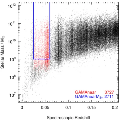
used throughout the remainder of this paper. Both GAMAnear and GAMAnearMlimare shown in redshift–stellar mass space in Fig.1.

3 S T E L L A R M A S S A N D M O R P H O L O G Y

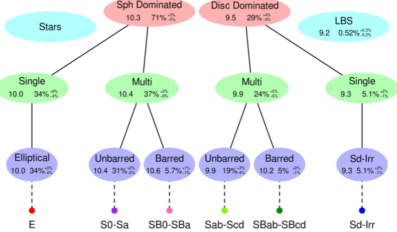
Fig. 2shows the stellar mass breakdown by type and morphol-ogy for the entirety of our mass limited sample of 2711 galaxies. Within each classification bubble, values for the logarithm of the median stellar mass (left) and the percentage by stellar mass with associated error (right) are shown. Percentage by stellar mass is cal-culated via a simple summation of theVmax-weighted stellar mass

of each galaxy within each population. Percentage errors represent the maximal dispersion between the three independent classifiers, i.e. the stellar mass for each galaxy population is rederived for each classifier and the offset from the master classification calculated. Note that the stellar masses for each galaxy as derived in Taylor et al. (2011) have a typical associated intrinsic stellar mass error of log(M_∗/M)∼0.1.

Approximately 71+₋34 per cent of the stellar mass in

our GAMAnearMlim sample is currently found within

at University of St Andrews on December 8, 2014

http://mnras.oxfordjournals.org/

Figure 1. Stellar mass as a function of redshift for galaxies within the GAMA survey. The red data points represent our GAMAnear sample; those galaxies that lie in the redshift range 0.025 < z < 0.06 with an associated GAMA redshift quality flag of nQ > 2 (i.e. good for science), an extinction corrected rband SDSS Petrosian magnitude of

r<19.4 mag and an absolute truncated S´ersic magnitude in therband ofMr<−17.4 mag. GAMAnear galaxies that additionally are more mas-sive than log(M_∗/M)>9.0 (within the blue box) constitute our stellar mass limited sample, GAMAnearMlim, in use throughout the remainder of this paper. Stellar masses shown here are notVmaxweight corrected. spheroid-dominated4 _{(elliptical and S0-Sa) systems, with the}

re-maining stellar mass in disc-dominated (Sab-Scd and Sd-Irr) galax-ies (29+₋₃4per cent) and LBS (∼0.52 per cent+₋₀0._.3₂). Adopting rea-sonable bulge-to-total values (e.g. for an intermediate Sb spiral, log (B/D)∼ −1, Graham & Worley2008) implies that approxi-mately half the stellar mass today resides in spheroidal structures,5

with the remaining half within disc-like structures, in-line with pre-vious studies (see Driver et al. 2007a,b; Gadotti2009; Tasca & White2011). Continuing further down the classification tree, we find approximate stellar mass proportions for E : S0-Sa : Sab-Scd : Sd-Irr of 34 : 37 : 24 : 5. For comparison, Table1shows the number fractions of various galaxy populations in stellar mass ranges with progressively more massive lower bounds. We see that no LBS-type galaxies exist in the mass range log(M_∗/M)>10.0. Spheroid-dominated galaxies become more numerous than disc-Spheroid-dominated galaxies at log(M_∗/M)>9.5, whilst elliptical galaxies alone dominate the galaxy population by number at log(M_∗/M)> 11.0. Interestingly, at stellar masses less massive than

4_{Here, the term ‘spheroid dominated’ does not refer to the spheroidal} com-ponent dominating the total flux of the system. As has been shown in Graham & Worley (2008), rarely does the spheroid component in a bulge+disc sys-tem contribute>50 per cent of the flux for galaxies later than S0. Rather, we define the term ‘spheroid dominated’ to refer to the visual impact of the spheroid on the postage stamp images presented in Kelvin et al. (2014); a combination of relative size, apparent surface brightness and 2D light profile.

5_{One expects the bulge-to-total ratio to correlate with the total stellar mass} of the system, and therefore, this value should be considered an estimate.

log(M∗/M)=11.0,∼25 per cent of the total galaxy population are consistently elliptical.

Our elliptical stellar mass fraction of 34 per cent+9₋₄is in excellent agreement with the value of 32 per cent found in Gadotti (2009)6

but significantly higher than the∼15 per cent value found in Driver et al. (2007b). This presumably reflects the great difficulty in dis-tinguishing between genuine pressure supported ellipticals and ro-tationally supported face-on lenticulars, as highlighted by the AT-LAS3D team, see for example Emsellem et al. (2011), Krajnovi´c et al. (2011), Cappellari et al. (2011b), Duc et al. (2011), Khochfar et al. (2011), also D’Onofrio et al. (1995); Graham et al. (1998). If the Driver et al. study is correct then the potential contamina-tion of our elliptical class by lenticular types may be significant. A key difference in our classifications and that of Driver et al. is the method of selection, with the former using eyeball morphology based on SDSS/UKIDSS data and the latter using GIM2D bulge– disc decompositions based on the significantly deeper Millennium Galaxy CatalogueB-band data (see Liske et al.2003; Driver et al. 2005). The Gadotti (2009) elliptical class is based on a Petrosian concentration index cut. In Driver et al. (2006) it was reported than the E/S0 (red spheroid) class contains (35±2) per cent of the stellar mass, which is closer to our elliptical value, and perhaps supporting the notion that our visually classified E class potentially contains a large fraction of lenticular contaminants. We will explore this issue in detail using robust structural decompositions (Kelvin et al., in preparation) based on theGALFITgalaxy fitting software (Peng et al. 2002, 2010a) and via ongoing Sydney-Australian-Astronomical-Observatory Multi-object Integral-Field Spectrograph (SAMI) and Calar Alto Legacy Integral Field spectroscopy Area survey (CALIFA) integral field unit observations (in progress). At present we advocate a small amount of caution in regards to the level of potential lenticular contamination of our elliptical sample.

4 T H E S T E L L A R M A S S F U N C T I O N

4.1 The galaxy stellar mass function

One of the most fundamental measurements in astronomy is that of the galaxy luminosity function, or its equivalent in mass, the GSMF. The GSMF gives the effective number of galaxies per unit volume in the logarithmic stellar mass interval logMto logM+d logM, where d logMis some log base 10 mass interval. Adopting the GAMA stellar masses presented in Taylor et al. (2011), we calculate our GSMF (and also our MSMFs below) via a direct summation of stellar mass in bins of 0.1 dex.

The GSMF may be described using a Schechter (1976) function whereby the number density,(logM)d logM, is given by

(logM)d logM=ln(10)·φ∗10log(M/M∗)(α+1)

×exp(−10log(M/M∗))d logM, (2)

whereM∗is the characteristic mass corresponding to the position of the distinctive ‘knee’ in the mass function. The termsα and φ∗ _{refer to the slope of the mass function at the low mass end}

and the normalization constant, respectively. Several recent stud-ies have previously measured the GSMF (e.g. Baldry et al.2008; Peng et al.2010b; Baldry et al.2012), and advocate the double Schechter form of the GSMF with a combined knee (M∗) for the

6_{Note that whilst the sample in Gadotti (2009) spans a similar redshift range,} their lower stellar mass limit is 1 dex higher, 1010_M

, than that adopted here.

at University of St Andrews on December 8, 2014

http://mnras.oxfordjournals.org/

Figure 2. The breakdown of stellar mass within our GAMAnearMlim sample by morphological type. Within each classification bubble, values for the logarithm of the median stellar mass (left) and the percentage of total stellar mass with its associated error (right) are shown. Stellar masses shown here have beenVmaxweight corrected.

Table 1. The number fractions of various galaxy populations for stellar mass ranges with progressively more massive lower bounds, as indicated. Barred populations have been merged into their sibling unbarred classes. Stellar masses shown here have beenVmaxweight corrected.

Population Stellar mass range [log(M∗/M)] >9 >9.5 >10 >10.5 >11 >11.5

LBS 0.04 0.01 0.00 0.00 0.00 0.00

E 0.19 0.24 0.24 0.31 0.72 1.00

S0-Sa 0.18 0.28 0.42 0.48 0.22 0.00 Sab-Scd 0.28 0.36 0.32 0.20 0.06 0.00 Sd-Irr 0.31 0.11 0.02 0.00 0.00 0.00 Sph dom 0.37 0.51 0.66 0.80 0.94 1.00 Disc dom 0.59 0.47 0.34 0.20 0.06 0.00

global population. The double-Schechter function is simply given bydouble(logM)d logM=1+2, where1and2refer to

equation (2) above, albeit with separate slope parameters,α1and

α2, and unique normalization values,φ1∗andφ∗2. Both1and2

share a commonM∗parameter. The double-Schechter function al-lows one to more accurately model the distinctive bump observed in the GSMF aboutM∗, with one Schechter function dominant at stellar masses greater thanM∗, and the second dominant oth-erwise. We adopt this technique, opting to fit the GSMF with a double Schechter model,7_{however, we maintain a single-Schechter}

model for the morphological-type stellar mass functions (MSMFs hereafter) that constitute it.

7_{All Schechter functions are fit using the}

NLMINBroutine in R; a quasi-Newton algorithm based on the PORT routines that optimize fitting in a similar sense to the Limited-memory Broyden–Fletcher–Goldfarb–Shanno algorithm (LM-BFGS), with an extension to handle simple box constraints on input variables (L-BFGS-B). The PORT documentation is available at

http://netlib.bell-labs.com/cm/cs/cstr/153.pdf

4.2 Morphological-type stellar mass functions

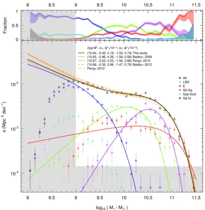
Fig.3shows our GSMF and constituent MSMFs for our volume and stellar mass limited GAMAnearMlimsample of 2711 systems.

Stellar masses shown here have beenVmaxweight corrected where

appropriate. The solid black line indicates a double Schechter fit to the total GSMF, binned into mass bins of 0.1 dex, whilst the various orange lines show similar GSMF double Schechter fits found in recent studies (Baldry et al.2008; Peng et al.2010b; Baldry et al. 2012; Peng et al.2012). Note that we choose not to match to ad-ditional complementary studies, such as that of Taylor et al. (2014, submitted) which divides their sample into statistically defined ‘R’ and ‘B’ populations, or the older yet still equally valid studies of Bell et al. (2003) and Baldry et al. (2004). This is for the sake of clarity alone, to avoid confusion within our Fig.3. Solid coloured lines indicate single-Schechter fits to the constituent MSMFs, where colour relates to morphology as indicated by the inset legend. Note that no Schechter fit to the LBS population is shown, as there was not sufficient data to constrain a Schechter function at this low mass end of the data set. Shaded grey areas (log(M_∗/M)<9.0 and number of galaxiesn≤3) indicate those regions where data has not been used in constraining the Schechter fits. Data points below our lower mass limit are from the parent GAMAnear sam-ple, and are shown only for reference. Also consider that the GAMA data set exhibits a high level of spectroscopic completeness (>98 per cent) down to its stated limiting apparent magnitude depth ofr=19.4 mag (Driver et al.2011), which precludes the possibility of severely impacting our measured stellar mass functions. The up-per panel of Fig.3shows the number fraction of galaxies as a func-tion ofVmaxweight corrected stellar mass, calculated in mass bins

identical to those in the lower panel. Shaded coloured regions around each morphological-type fraction line within the upper panel indi-cate the±1σ confidence intervals, as calculated using theQBETA

function (Cameron2011).

We find our global GSMF in excellent agreement with the complementary studies shown in Fig.3, exhibiting a comparable

at University of St Andrews on December 8, 2014

http://mnras.oxfordjournals.org/

Figure 3. The GSMF and constituent MSMFs as fit by double and single-Schechter functions, respectively. Each galaxy population is labelled and coloured according to the inset legend. The data are split into mass bins of 0.1 dex, with the error per bin assumed to be Poissonian (√n) in nature. Shaded grey areas (log(M_∗/M)<9.0 and number of galaxiesn≤3) indicate those regions where data have not been used in constraining the Schechter fits. Schechter fit parameters for the GSMF in addition to fits from other studies are also shown for reference. The upper panel shows the number fraction of galaxies as a function ofVmaxweight corrected stellar mass, calculated in mass bins identical to those in the lower panel. Shaded coloured regions around each morphological-type fraction line indicate the±1σconfidence intervals, as calculated using theQBETAfunction (Cameron2011).

M∗_{Schechter fit parameter at log(M}∗_{/M)=10.64±0.07, and}

agreeing well within the errors. The high-mass end of our sample predominantly consists of spheroid-dominated elliptical and S0-Sa type galaxies. At intermediate masses below the globalM∗value, the disc-dominated Sab-Scd population dominates the stellar mass budget, whilst at the low mass end of our data set the Sd-Irr and LBS populations are the most influential. It is apparent that the latter LBS population is poorly sampled in this mass regime, with the M∗ parameter likely residing below our lower stellar mass limit of log(M_∗/M)=9.0. For this reason, we do not provide Schechter function fit parameters to the LBS population in this study. We remind the reader that this sample should be considered a field-dominated sample, rather than a cluster environment, as is

evidenced by the dominance of Sd-Irr and LBS type systems at the low mass end of our data set.

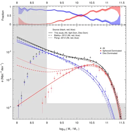
Because of the uncertainty in our elliptical/S0-Sa division, and in an attempt to group galaxies into structurally meaningful parent samples, we now also combine our morphological types into two populations in Fig.4as indicated, namely: spheroid-dominated (E, S0-Sa) and disc-dominated (Sab-Scd, Sd-Irr) galaxies, and simi-larly fit these data with a single-Schechter function. our recovered

M∗_{Schechter fit parameters for our combined stellar mass}

func-tions are remarkably similar to one another and to our total GSMF, with log(M∗/M)=10.60 and 10.70, respectively, supporting the notion that the combined total GSMF is well described by a double-Schechter function comprised of two distinct components identified

at University of St Andrews on December 8, 2014

http://mnras.oxfordjournals.org/

Figure 4. As Fig.3, but for a reduced grouping of morphological types, as indicated, which may broadly be compared to early-type and late-type galaxies. Comparison of Schechter function fits for similar red and blue populations from Baldry et al. (2012) and Peng et al. (2012) are also shown.

morphologically here. Comparison of Schechter function fits for a similar red and blue population from Baldry et al. (2012) and Peng et al. (2012) are also shown in Fig. 4. The Peng et al. GSMF is a summation of Schechter function fits to red/blue central and red/blue satellite galaxies. We find our disc-dominated population in excellent agreement with the Baldry et al. and Peng et al. blue populations, agreeing well at the lowest stellar masses, whilst we find a slight surplus of stellar mass in disc-dominated galaxies at masses greater thanM∗. Our spheroid-dominated population simi-larly shows good level of agreement at the most massive end of our sample beyondM∗; however, we do not find the low-mass turn up found in the comparison red populations.

The cause of this discrepancy remains somewhat a mystery, and perhaps rests with our choice of comparison samples. For exam-ple, Yang, Mo & van den Bosch (2009) find no low-mass turn up for their red population across a stellar mass regime comparable to that probed here, disagreeing with the studies above, and

highlight-ing apparent difficulties when dividhighlight-ing the galaxy population by colour alone. Similarly, whilst Muzzin et al. (2013) and Tomczak et al. (2014) do find a low-mass turn up in the stellar mass func-tion of quiescent galaxies when dividing the galaxy populafunc-tion into quiescent/star-forming sub-populations, Omand, Balogh & Pog-gianti (2014) find no noticeable low-mass turn up for their equiv-alent quiescent sample. To expand on the relation between colour and stellar mass, Fig.5shows global rest-frame colour, (g−i)rest,

as a function of galaxy stellar mass, log(M_∗/M). Our rest-frame colours are those derived concurrently with the stellar masses from Taylor et al. (2011), i.e. an Spectral Energy Distribution (SED) fit to the GAMA galaxy photometry. The top left-hand panel dis-plays several overlaid contour maps highlighting the population density in colour–mass space for all of our morphological types, as indicated by the inset legend, whereas the remaining panels repre-sent the same colour–mass space for each population in isolation, as labelled in the top-left corner of each panel. For these latter

at University of St Andrews on December 8, 2014

http://mnras.oxfordjournals.org/

Figure 5. Global rest-frame colour, (g−i)rest, as a function ofVmaxweight corrected galaxy stellar mass, log(M∗/M). The top left panel displays several overlaid contour maps highlighting the population density in colour–mass space for each of our morphological types, as indicated by the inset legend. Contours represent 5, 10, 20, 40 and 80 per cent of the peak total population density. The shaded grey area at log(M_∗/M)<9.0 represents the region in which our data becomes stellar mass incomplete. The remaining panels represent a similar colour–mass space but for each population in isolation, as labelled in the top-left corner of each panel. For each panel, we display a three-colour (RGB=Hig) postage stamp image of a galaxy at each position within a grid of bin sizes 0.1 in stellar mass and 0.03 in colour. Each postage stamp is approximately 7 arcsec×7 arcsec in size. Blank spaces indicate a grid element where no galaxy of that morphological class exists.

at University of St Andrews on December 8, 2014

http://mnras.oxfordjournals.org/

panels, we display a three-colour (RGB= Hig)8 _{postage stamp}

image of a galaxy at each position within a grid of bin size 0.1 in stellar mass and 0.03 in colour, where a blank space indicates no galaxy of that morphological type exists. In total in this figure, we display 1245 galaxies from our GAMAnear sample (32.5 per cent), with each postage stamp approximately 7 arcsec×7 arcsec in size. We find the spheroid-dominated elliptical and lenticular/early-type red sequence extending across a wide range of stellar masses, 9.5<log(M∗/M)<11.5 with a relatively small variation in global (g − i)rest colour across this range. As can also be seen

in Fig.3, the elliptical population rarely dominates the stellar mass budget in this range for any given stellar mass, except at the most massive extreme of our sample (log(M_∗/M)∼11). At stellar masses below log(M_∗/M)≈10.2, first the disc-dominated Sab-Scd population followed by the Sd-Irr population provide a signifi-cant contamination fraction to the red sequence. This contamination ‘break-point’ is in good agreement with that reported in Taylor et al. (2014, submitted), whereby the mean colour of a statistically de-fined red population of galaxies jumps by≈0.2 mag, coupled with an increase in scatter, at log(M∗/M)≈10.1.

One possible explanation behind this red sequence contamination becomes apparent in the postage stamps for the Sab-Scd and Sd-Irr population panels. In the colour regime (g−i)rest>0.7, a significant

fraction of disc-dominated galaxies are observed highly inclined or edge on. The reprocessing of galactic light as it travels through a disc has the effect of reddening the resultant light due to the effects of intrinsic dust attenuation, so therefore any photometric estimate of the global colour will be biased redwards, in addition to affecting other measured photometric properties (e.g. Pastrav et al.2013). This late-type morphological contamination of the red sequence, effectively a redistribution of stellar mass from the blue to the red population, may perhaps be responsible for the observed turn up of the red population stellar mass functions at the low mass end reported in, e.g. Baldry et al. (2012), Peng et al. (2012). Further, we posit that any such division of the local galaxy population by (uncorrected) colour into a red sequence and blue cloud, such as that adopted by, e.g. Bell et al. (2003), Baldry et al. (2004) – a division in colour–magnitude space – and Peng et al. (2010b) – a division in colour–stellar mass space – becomes increasingly meaningless at stellar masses below log(M_∗/M)≈10.2.

We stress however that colour is no more equivalent to spheroid/disc-dominated than it is to quiescent/star-forming, slow/fast rotator, early-type/late-type or metal rich/poor, to name but a few common bimodal galaxy identities. Whilst significant overlaps may, and do, exist between these populations, they do in fact measure distinct galaxy populations, and therefore one may not always expect to recover a similar trend in, for example, the observed stellar mass function. Also consider that our choice to construct a spheroid-dominated sample from elliptical and S0-Sa galaxies alone undoubtedly influences our recovered stellar mass functions. We note that, should we choose to include the LBS popu-lation into the spheroid-dominated popupopu-lation, we similarly recover a low-mass turn up such as that observed in Baldry et al. (2012) and Peng et al. (2012). However, since LBS galaxies are notably blue, one might expect any division by colour to bin LBS galaxies with

8_{Postage stamps of a peculiar turquoise colour indicate galaxies that lie in} a region where no near-infrared (UKIDSS-LAS) data were available at the time of postage stamp creation, hence a missing red channel in the creation of our three-colour images.

our typically blue disc-dominated systems, increasing the number density for the disc-dominated population alone, and therefore not providing the required turn-up for spheroid-dominated systems in the low-mass regime. See Appendix A for a further discussion of the inclusion of the LBS population into our spheroid-dominated class.

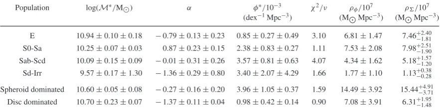
Full Schechter fit parameters for both the double GSMF and constituent MSMFs (both Hubble-type morphologies and combined spheroid/disc-dominated populations) are shown in Tables2and3, respectively. As previously noted, we do not provide Schechter fit parameters for the LBS population. Errors on theρparameter are propagated through from the stellar mass errors estimated in Taylor et al. (2011), typically of the order∼0.1 dex. The second set of errors for the logM∗,αandφ∗parameters represent one standard deviation as derived from comparable Schechter function fits to each individual observers data set alone, giving an indication of classification agreement between all three observers. All other errors provided in both tables are estimated from jackknifed resampling using the relationσ2₌ N−1

N

_N

i=1(xj−x)

2_{, where xis the}

best-fitting parameter,xjis the best-fitting parameter as given from a jackknife resampled variant of the data set andN represents the number of jackknife volumes (we adoptN=10).

The double Schechter GSMF provides a good fit to the bimodal form of the total population, with a goodness of fit parameter of χ2_{/ν=1.12 (aχ}2_{p-value ofp=0.33, withχ}2_{=21.2 andk=19}

degrees of freedom; i.e. we have insufficient evidence to reject our fitted model). As can be inferred from Fig.3and the gradient of the elliptical population in Table3, the initial high-mass peak primarily consists of S0-Sa galaxies, with some small contribution from el-liptical galaxies. Elel-lipticals appear to exist uniformly across a wide range of masses. Our fitted Schechter function to the elliptical pop-ulation appears to be a relatively poor fit to the data, as evidenced by the goodness of fit parameter and confidence intervals quoted in Table3, able to capture the high-mass turnover aboutM∗but par-tially underestimating the number counts at lower stellar masses. No doubt this discrepancy is caused by the inflexibility of the Schechter function in fitting a population that is uniformly distributed in num-ber density such as this. Similarly, the goodness of fit parameter for the Sab-Scd population is quite poor. From Fig.3, we see that this discrepancy occurs at the high-mass end, aboveM∗, with an unex-pected surplus of galaxies and a departure from the Schechter fit at log(M∗/M)∼11. This could be evidence of perhaps spheroid-dominated (elliptical, lenticular or early-type spiral) contamination of the Sab-Scd population in this regime. In addition, errors arising from observer disagreement place a significant level of uncertainty on Schechter fit parameters to our Sd-Irr population. This implies that perhaps these data are not of a sufficient depth to fully mea-sure the characteristic turnover in the Sd-Irr stellar mass function. Visual classification error for the remaining morphological types remains minimal however, typically of the order of or less than the quoted standard errors. We find that our recoveredM∗parameter for our constituent MSMFs decrease systematically from spheroid-dominated to disc-spheroid-dominated galaxies; for E, S0-Sa, Sab-Scd and Sd-Irr type galaxies we find log(M∗/M)=10.94, 10.25, 10.09, 9.57.

Our combined spheroid-dominated and disc-dominated single-Schechter fits provide an excellent description of the spheroid and disc-dominated galaxy populations. The goodness of fit es-timators both indicate the Schechter model is able to adequately and accurately reproduce the distribution observed in the data, whilst the quoted errors, both standard and visual, remain low.

at University of St Andrews on December 8, 2014

http://mnras.oxfordjournals.org/

Table 2. Double Schechter stellar mass function fit parameters for the total GSMF as shown in Fig.3. From left to right, columns are: the shared knee in the Schechter function (M∗); the primary slope of the faint end of the Schechter function (α1); the primary normalization constant for the Schechter function (φ₁∗); the secondary slope of the faint end of the Schechter function (α2); the secondary normalization constant for the Schechter function (φ∗₂); theχ2_{goodness of fit parameter (χ}2_{/ν); the stellar mass density} implied in the usual way via the fitted Schechter function [ρ_φ=N_i=1φ_i∗M∗(αi+2)]; the stellar mass density calculated via the direct summation of the stellar masses from the individual galaxies [ρ=_V1Ni=1M∗]. The double-Schechter function is fit to

N=24 data bins withn=5 fitted parameters, therefore, the number of degrees of freedom for this fit is given byν=N−n=19. log(M∗/M) α1 φ1∗/10−3 α2 φ∗2/10−3 χ2/ν δφ/107 δ/107

(dex−1_Mpc−3_{) (dex}−1_Mpc−3_{) (M}

Mpc−3_{) (M}

Mpc−3₎ 10.64±0.07 −0.43±0.35 4.18±1.52 −1.50±0.22 0.74±1.13 1.12 22.07±7.91 21.88+₋6₅._.90₂₂

Table 3. As Table2, but single-Schechter stellar mass function fit parameters for the MSMFs in Figs3and4. The second set of confidence intervals for the logM∗,αandφ∗parameters indicate one standard deviation as determined from single-Schechter fits to each individual observers data sets. These single-Schechter functions are fit toN=24 data bins withn=3 fitted parameters, therefore, the number of degrees of freedom for this fit is given byν=N−n=21.

Population log(M∗/M) α φ∗/10−3 _χ2_{/ν ρ}

φ/107 _ρ

/107 (dex−1_Mpc−3_{) (M}

Mpc−3_{) (M}

Mpc−3₎ E 10.94±0.10±0.18 −0.79±0.13±0.23 0.85±0.27±0.49 3.10 6.81±1.47 7.46+₋21..4081 S0-Sa 10.25±0.07±0.03 0.87±0.23±0.15 2.38±0.83±0.27 1.11 7.53±2.08 7.98+₋2₁._.51₉₀ Sab-Scd 10.09±0.15±0.09 −0.01±0.31±0.26 3.57±0.81±0.63 4.07 4.34±1.62 5.18+₋1₁._.57₂₀ Sd-Irr 9.57±0.17±1.30 −1.36±0.29±0.80 3.40±2.07±4.29 1.66 1.77±1.10 1.13+₋0₀._.38₂₈ Spheroid dominated 10.60±0.05±0.08 −0.27±0.16±0.20 3.96±1.05±0.37 1.59 14.49±3.92 15.44+₋4₃._.91₇₁

Disc dominated 10.70±0.23±0.07 −1.37±0.11±0.04 0.98±0.42±0.14 0.90 7.08±3.91 6.31+₋1₁._.95₄₈

Further, we note that the recovered Schechter fit parameters to our spheroid-dominated and disc-dominated populations: logM∗= 10.60, 10.70;α= −0.27,−1.37, andφ∗=3.96, 0.98, respectively, are in good agreement with those found for our double Schechter fit to the total population: logM∗=10.64, 10.64;α= −0.43,−1.50; φ∗_{= 4.18, 0.74. The apparent self-similarity between these two}

sets of recovered parameters supports the notion that our division of the GSMF into spheroid-dominated and disc-dominated sub-populations is indeed physically meaningful. By dividing galaxies according to their dominant structural component, we have been able to naturally recover the fundamental parameters which best describe the full stellar mass distribution of galaxies in the local Universe.

5 C O N C L U S I O N S

We have analysed a morphologically classified sample of 2711 galaxies selected from the GAMA survey by virtue of their redshift range (0.025 < z < 0.06) and global stellar mass (log(M∗/M)>9.0). Each galaxy is classified into either ellipti-cal (E), spheroid-dominated lenticular and early-type spiral (S0-Sa), intermediate/late-type spiral (Sab-Scd) and a disc-dominated or ir-regular (Sd-Irr) class. Within this local sample, we find approximate stellar mass proportions for E : S0-Sa : Sab-Scd : Sd-Irr of 34 : 37 : 24 : 5, acknowledging a potential cross-contamination between our elliptical and S0-Sa classes. We find that colour and mass cuts do not trivially recover Hubble-type classifications and advocate against using ‘red’ and ‘blue’ terminology interchangeably with ‘early’ and ‘late’, or ‘spheroid dominated’ and ‘disc dominated’ as these are clearly very different distinctions. Grouping by the dom-inant structural component, spheroid or disc, we further find that approximately 71+₋34per cent of the stellar mass is currently found

within spheroid-dominated elliptical and S0-Sa type galaxies, with

29+4₋₃per cent residing in disc-dominated Sab-Scd and Sd-Irr sys-tems. Adopting reasonable bulge-to-total values (e.g. Graham & Worley2008) implies that approximately half the stellar mass to-day resides in spheroidal structures, with the remaining half within disc-like structures, in-line with previous studies (see Driver et al. 2007a,b; Gadotti2009; Tasca & White2011).

The total GSMF for our sample is well described by a double-Schechter function with parameters M∗=1010.64_M

, α1 = −0.43, φ∗1=4.18 dex−

1

Mpc−3, α2 = −1.50 and φ2∗=

0.74 dex−1Mpc−3. The constituent MSMFs are well sampled above our lower stellar mass limit, with the exception of the LBS pop-ulation, which remains incomplete down to log(M_∗/M)∼9.0. Each MSMF is adequately described by a single-Schechter function (Fig.3), with a notable underestimation of the number density of el-liptical galaxies at low stellar masses (log(M_∗/M)<10), and an underestimation of our Sab-Scd population number density at high stellar masses (log(M_∗/M)∼11). We find our recoveredM∗for these MSMFs decreases systematically from spheroid-dominated to disc-dominated galaxies, i.e. for E, S0-Sa, Sab-Scd and Sd-Irr type galaxies we find log(M∗/M)=10.94, 10.25, 10.09, 9.57, respectively.

Our combined spheroid-dominated and disc-dominated stellar mass functions are each well described by a single-Schechter function (Fig.4). Interestingly, our recoveredM∗parameters for our combined spheroid-dominated and disc-dominated stellar mass functions are remarkably similar to one another, in addition to our total GSMF, with log(M∗/M)=10.60 and 10.70, respec-tively, as compared with log(M∗/M)=10.64. We also find a good level of agreement between our spheroid and disc-dominated populations and the total GSMF for the additional Schechter fit parameters,αandφ∗. That these two sets of values should arise naturally from the data supports the notion that the combined to-tal GSMF is indeed comprised of two complementary, yet distinct,

at University of St Andrews on December 8, 2014

http://mnras.oxfordjournals.org/

sub-populations, each best described according to their dominant structural component. We find that the discrepancy between our spheroid-dominated stellar mass function and the comparison red sequence stellar mass functions of Baldry et al. (2012) and Peng et al. (2012) at the low-mass end of our sample can potentially be attributed to late-type contamination of the red sequence (Fig.5), although we note that a division of the local galaxy population by colour may not easily be comparable to a division by dominant structural component; nor should it. In addition, the inclusion of the LBS population into the spheroid-dominated class acts to remove the observed low-mass discrepancy, however, it is not clear that this inclusion is desired. Therefore, in conclusion, our campaign of robust morphological classification shows that the local GSMF is adequately described by a double-Schechter function comprised of two distinct populations: spheroid-dominated and disc-dominated galaxies.

AC K N OW L E D G E M E N T S

This work was supported by the Austrian Science Foundation FWF under grant P23946. AWG was supported under the Australian Research Council’s funding scheme FT110100263. GAMA is a joint European-Australasian project based around a spectroscopic campaign using the Anglo-Australian Telescope. The GAMA input catalogue is based on data taken from the Sloan Digital Sky Survey and the UKIRT Infrared Deep Sky Survey. Complementary imaging of the GAMA regions is being obtained by a number of independent survey programmes including GALEXMIS, VST KiDS, VISTA VIKING,WISE,Herschel-ATLAS, GMRT and ASKAP providing UV to radio coverage. GAMA is funded by the STFC (UK), the ARC (Australia), the AAO, and the participating institutions. The GAMA website ishttp://www.gama-survey.org/.

R E F E R E N C E S

Abazajian K. N. et al., 2009, ApJS, 182, 543

Allen P. D., Driver S. P., Graham A. W., Cameron E., Liske J., de Propris R., 2006, MNRAS, 371, 2

Baldry I. K., Glazebrook K., Brinkmann J., Ivezi´c ˇZ., Lupton R. H., Nichol R. C., Szalay A. S., 2004, ApJ, 600, 681

Baldry I. K., Balogh M. L., Bower R. G., Glazebrook K., Nichol R. C., Bamford S. P., Budavari T., 2006, MNRAS, 373, 469

Baldry I. K., Glazebrook K., Driver S. P., 2008, MNRAS, 388, 945 Baldry I. K. et al., 2010, MNRAS, 404, 86

Baldry I. K. et al., 2012, MNRAS, 421, 621 Bamford S. P. et al., 2009, MNRAS, 393, 1324

Behroozi P. S., Wechsler R. H., Conroy C., 2013, ApJ, 770, 57

Bell E. F., McIntosh D. H., Katz N., Weinberg M. D., 2003, ApJS, 149, 289

Blanton M. R., Eisenstein D., Hogg D. W., Schlegel D. J., Brinkmann J., 2005, ApJ, 629, 143

Bolzonella M. et al., 2010, A&A, 524, A76 Bruzual G., Charlot S., 2003, MNRAS, 344, 1000 Bundy K. et al., 2010, ApJ, 719, 1969

Calzetti D., Armus L., Bohlin R. C., Kinney A. L., Koornneef J., Storchi-Bergmann T., 2000, ApJ, 533, 682

Cameron E., 2011, Publ. Astron. Soc. Aust., 28, 128

Caon N., Capaccioli M., D’Onofrio M., 1993, MNRAS, 265, 1013 Cappellari M. et al., 2011a, MNRAS, 413, 813

Cappellari M. et al., 2011b, MNRAS, 416, 1680 Cappellari M. et al., 2013, MNRAS, 432, 1862 Chabrier G., 2003, PASP, 115, 763

Conselice C. J., 2006, MNRAS, 373, 1389

Cook M., Lapi A., Granato G. L., 2009, MNRAS, 397, 534

Cook M., Evoli C., Barausse E., Granato G. L., Lapi A., 2010, MNRAS, 402, 941

Cooper M. C. et al., 2012, MNRAS, 419, 3018

D’Onofrio M., Zaggia S. R., Longo G., Caon N., Capaccioli M., 1995, A&A, 296, 319

Davies R. L., Illingworth G., 1983, ApJ, 266, 516

Davies R. L., Efstathiou G., Fall S. M., Illingworth G., Schechter P. L., 1983, ApJ, 266, 41

De Lucia G., Blaizot J., 2007, MNRAS, 375, 2

De Lucia G., Kauffmann G., White S. D. M., 2004, MNRAS, 349, 1101 Debattista V. P., Mayer L., Carollo C. M., Moore B., Wadsley J., Quinn T.,

2006, ApJ, 645, 209

Driver S. P., Liske J., Cross N. J. G., De Propris R., Allen P. D., 2005, MNRAS, 360, 81

Driver S. P. et al., 2006, MNRAS, 368, 414

Driver S. P., Popescu C. C., Tuffs R. J., Liske J., Graham A. W., Allen P. D., de Propris R., 2007a, MNRAS, 379, 1022

Driver S. P., Allen P. D., Liske J., Graham A. W., 2007b, ApJ, 657, L85 Driver S. P. et al., 2009, Astron. Geophys., 50, 050000

Driver S. P. et al., 2011, MNRAS, 413, 971

Driver S. P., Robotham A. S. G., Bland-Hawthorn J., Brown M., Hopkins A., Liske J., Phillipps S., Wilkins S., 2013, MNRAS, 430, 2622 Duc P.-A. et al., 2011, MNRAS, 417, 863

Emsellem E. et al., 2011, MNRAS, 414, 888 Gadotti D. A., 2009, MNRAS, 393, 1531

Graham A. W., Driver S. P., 2005, Publ. Astron. Soc. Aust., 22, 118 Graham A. W., Worley C. C., 2008, MNRAS, 388, 1708

Graham A. W., Colless M. M., Busarello G., Zaggia S., Longo G., 1998, A&AS, 133, 325

Graham A. W., Merritt D., Moore B., Diemand J., Terzi´c B., 2006, AJ, 132, 2711

Hill D. T. et al., 2011, MNRAS, 412, 765 Kauffmann G. et al., 2003, MNRAS, 341, 54

Kauffmann G., White S. D. M., Heckman T. M., M´enard B., Brinchmann J., Charlot S., Tremonti C., Brinkmann J., 2004, MNRAS, 353, 713 Kelvin L., Driver S., Robotham A., Hill D., Cameron E., 2010, in Debattista

V. P., Popescu C. C., eds, AIP Conf. Proc. Vol. 1240, Hunting for The Dark: The Hidden Side of Galaxy Formation. Am. Inst. Phys., New York, p. 247

Kelvin L. S. et al., 2012, MNRAS, 421, 1007 Kelvin L. S. et al., 2014, MNRAS, 439, 1245

Kereˇs D., Katz N., Weinberg D. H., Dav´e R., 2005, MNRAS, 363, 2 Khochfar S., Silk J., 2006a, MNRAS, 370, 902

Khochfar S., Silk J., 2006b, ApJ, 648, L21 Khochfar S. et al., 2011, MNRAS, 417, 845 Kormendy J., Bender R., 2012, ApJS, 198, 2 Krajnovi´c D. et al., 2011, MNRAS, 414, 2923

L’Huillier B., Combes F., Semelin B., 2012, A&A, 544, A68 Lara-L´opez M. A. et al., 2010, A&A, 521, L53

Lara-L´opez M. A. et al., 2013, MNRAS, 434, 451 Lawrence A. et al., 2007, MNRAS, 379, 1599

Liske J., Lemon D. J., Driver S. P., Cross N. J. G., Couch W. J., 2003, MNRAS, 344, 307

Matkovi´c A., Guzm´an R., 2005, MNRAS, 362, 289 Moustakas J. et al., 2013, ApJ, 767, 50

Muzzin A. et al., 2013, ApJ, 777, 18 Navarro J. F., Benz W., 1991, ApJ, 380, 320

Omand C., Balogh M., Poggianti B., 2014, MNRAS, 440, 843

Pastrav B. A., Popescu C. C., Tuffs R. J., Sansom A. E., 2013, A&A, 553, A80

Patel S. G. et al., 2013, ApJ, 766, 15

Peng C. Y., Ho L. C., Impey C. D., Rix H.-W., 2002, AJ, 124, 266 Peng C. Y., Ho L. C., Impey C. D., Rix H.-W., 2010a, AJ, 139, 2097 Peng Y.-j. et al., 2010b, ApJ, 721, 193

Peng Y.-j., Lilly S. J., Renzini A., Carollo M., 2012, ApJ, 757, 4

Pichon C., Pogosyan D., Kimm T., Slyz A., Devriendt J., Dubois Y., 2011, MNRAS, 418, 2493

Pozzetti L. et al., 2010, A&A, 523, A13

at University of St Andrews on December 8, 2014

http://mnras.oxfordjournals.org/

Robotham A. S. G. et al., 2011, MNRAS, 416, 2640 Robotham A. S. G. et al., 2013, MNRAS, 431, 167 Schechter P., 1976, ApJ, 203, 297

Schmidt M., 1968, ApJ, 151, 393

S´ersic J. L., 1963, Bol. Asociacion Argentina Astron. La Plata Argentina, 6, 41

Shankar F., Marulli F., Bernardi M., Mei S., Meert A., Vikram V., 2013, MNRAS, 428, 109

Shen S., Mo H. J., White S. D. M., Blanton M. R., Kauffmann G., Voges W., Brinkmann J., Csabai I., 2003, MNRAS, 343, 978

Shimizu I., Inoue A. K., 2013, PASJ, 65, 96

Simard L., Mendel J. T., Patton D. R., Ellison S. L., McConnachie A. W., 2011, ApJS, 196, 11

Szomoru D., Franx M., van Dokkum P. G., Trenti M., Illingworth G. D., Labb´e I., Oesch P., 2013, ApJ, 763, 73

Tasca L. A. M., White S. D. M., 2011, A&A, 530, A106 Taylor E. N. et al., 2011, MNRAS, 418, 1587

Tomczak A. R. et al., 2014, ApJ, 783, 85 Tremonti C. A. et al., 2004, ApJ, 613, 898

van den Bosch F. C., Aquino D., Yang X., Mo H. J., Pasquali A., McIntosh D. H., Weinmann S. M., Kang X., 2008, MNRAS, 387, 79

van Dokkum P. G. et al., 2010, ApJ, 709, 1018 White S. D. M., Frenk C. S., 1991, ApJ, 379, 52

Wyse R. F. G., Gilmore G., Franx M., 1997, ARA&A, 35, 637 Yang X., Mo H. J., van den Bosch F. C., 2009, ApJ, 695, 900 York D. G. et al., 2000, AJ, 120, 1579

Young C. K., Currie M. J., 1994, MNRAS, 268, L11

A P P E N D I X A : I M PAC T O F T H E L B S P O P U L AT I O N O N T H E G S M F

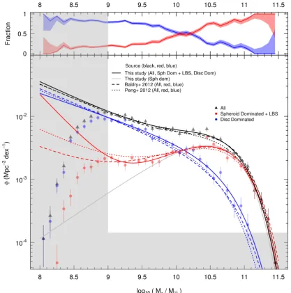
Our prior division of our galaxy sample into spheroid-dominated (E, S0-Sa) and disc-dominated (Sab-Scd, Sd-Irr) galaxies, as shown in Fig.4, neglected the low-mass LBS population. Fig.A1shows the GSMF and disc-dominated MSMF as before, but with an updated spheroid-dominated MSMF including the LBS population (i.e. E,

Figure A1. As Fig.4, but with the inclusion of the LBS population in the spheroid-dominated class (red data points). The combined spheroid-dominated plus LBS population is fitted by a double Schechter component (red solid line) as is the total galaxy population (solid black line), whereas the disc-dominated population remains well described by a single-Schechter function (solid blue line). The previous spheroid-dominated (E, S0-Sa) single-Schechter function fit is shown in light grey, for reference. Comparison of Schechter function fits for similar red and blue populations from Baldry et al. (2012) and Peng et al. (2012) are also shown.

at University of St Andrews on December 8, 2014

http://mnras.oxfordjournals.org/

Table A1. Double Schechter stellar mass function fit parameters for the combined spheroid-dominated plus LBS galaxy population as shown in Fig.A1. From left to right, columns are: the shared knee in the Schechter function (M∗); the primary slope of the faint end of the Schechter function (α1); the primary normalization constant for the Schechter function fit (φ1∗); the secondary slope of the faint end of the Schechter function (α2); the secondary normalization constant for the Schechter function fit (φ∗2); theχ2goodness of fit parameter (χ2_{/ν); the stellar mass density implied in the usual way via the fitted Schechter function [ρ}

φ=Ni=1φ_i∗M∗(αi+2)]; the stellar mass density calculated via the direct summation of the stellar masses from the individual galaxies [ρ= _V1 Ni=1M∗]. The double-Schechter function is fit toN=24 data bins withn=5 fitted parameters, therefore, the number of degrees of freedom for this fit is given byν=N−n=19.

log(M∗/M) α1 φ1∗/10−3 α2 φ2∗/10−3 χ2/ν δφ/107 δ/107 (dex−1_Mpc−3_{) (dex}−1_Mpc−3_{) (M}

Mpc−3_{) (M}

Mpc−3₎ 10.65±0.08 −0.37±0.23 3.63±1.38 −2.13±1.23 0.01±0.05 0.96 14.29±7.76 15.56+₋4₃._.95₇₄

S0-Sa, LBS). All data analysis is conducted in a similar fashion to that outlined in Section 4. The previous spheroid-dominated (E, S0-Sa) single-Schechter function fit is shown in light grey, for reference. As can clearly be seen, once the LBS galaxy population is included into the spheroid-dominated class, we recover a low-mass upturn exceedingly similar in nature to the red population as reported in, e.g. Baldry et al. (2012) and Peng et al. (2012). On the surface, the spheroid-dominated class may perhaps be the natural home of the ‘LBS’ galaxy population, allowing us to maintain a good level of agreement with comparison studies.

However, we remind the reader that our adopted visual morpho-logical classification boundaries (Kelvin et al.2014) are substan-tially different from the red/blue divisions presented in Baldry et al. (2012) and Peng et al. (2012), and also the star-forming/quiescent divisions as noted in Section 4.2. See, for example, Fig.5for a visual representation of the colour mix across all morphologies. Indeed, despite the inherent trends between morphology, colour and star formation rate, we see no explicit reason why a bimodal division along morphological lines should reproduce exactly that of one which has been created along colour or star formation rate measures. In which case, it is perhaps surprising that a combined spheroid-dominated plus LBS population so closely recovers the low-mass upturn observed in the red populations of Baldry et al. (2012) and Peng et al. (2012). Also note that whilst the third word in LBS denotes its shape, the second part of the acronym denotes their typical colour: blue. As is shown in Fig.5, the majority of blue galaxies lie in the disc-dominated Sab-Scd and Sd-Irr classes, giving weight to the inclusion of the LBS population in our disc-dominated sub-sample instead. This would only serve to increase the low-mass upturn of the disc-dominated population, and maintain the low-mass discrepancy we observe between our spheroid-dominated class and the comparison red-population data from the literature. The correct placement of our LBS galaxy population within the morpholog-ical schema adopted throughout this study remains unclear, and therefore, we continue to advocate its exclusion at present. Future studies are planned to clarify the importance of the LBS population (Moffett et al., in preparation).

TableA1provides the double Schechter fit parameters to the com-bined spheroid-dominated (E, S0-Sa) plus LBS population. Note the unusually lowα2slope parameter, combined with relatively large

error bars. This indicates that shape of the low-mass end of our Schechter fit is poorly constrained, as is evidenced by the unusually

steep gradient of the fit when extrapolated below our mass limit (see Fig.A1). Nevertheless, the Schechter fit provides a good descrip-tion of the data across the range of interest (log(M_∗/M)>9.0), exhibiting a strong goodness of fit parameter.

1_{Institut f¨ur Astro- und Teilchenphysik, Universit¨at Innsbruck,}

Techniker-straße 25, A-6020 Innsbruck, Austria

2_{School of Physics and Astronomy, University of St Andrews, North Haugh,}

St Andrews, Fife KY16 9SS, UK

3_{International Centre for Radio Astronomy Research, 7 Fairway, The}

Uni-versity of Western Australia, Crawley, Perth, WA 6009, Australia

4_{School of Physics, the University of Melbourne, Parkville, VIC 3010,}

Aus-tralia

5_{Centre for Astrophysics and Supercomputing, Swinburne University of}

Technology, Hawthorn, VIC 3122, Australia

6_{Astrophysics Research Institute, Liverpool John Moores University, Twelve}

Quays House, Egerton Wharf, Birkenhead CH41 1LD, UK

7_{School of Physics and Astronomy, The University of Nottingham, University}

Park, Nottingham NG7 2RD, UK

8_{Australian Astronomical Observatory, PO Box 915, North Ryde, NSW 1670,}

Australia

9_{Sydney Institute for Astronomy, School of Physics A28, University of Sydney,}

NSW 2006, Australia

10_{School of Physics, Monash University, Clayton, VIC 3800, Australia} 11_{Research School of Astronomy and Astrophysics, The Australian National}

University, Canberra, ACT 2611, Australia

12_{European Space Agency, ESTEC, Keplerlaan 1, NL-2200 AG Noordwijk,}

the Netherlands

13_{European Southern Observatory, Karl-Schwarzschild-Str. 2, D-85748}

Garching, Germany

14_{Department of Physics and Astronomy, Macquarie University, NSW 2109,}

Australia

15_{Astronomy Centre, University of Sussex, Falmer, Brighton BN1 9QH, UK} 16_{Institute for Computational Cosmology, Department of Physics, Durham}

University, South Road, Durham DH1 3LE, UK

17_{Astrophysics Group, HH Wills Physics Laboratory, University of Bristol,}

Tyndall Avenue, Bristol BS8 1TL, UK

18_{Jeremiah Horrocks Institute, School of Computing, Engineering and}

Phys-ical Sciences, University of Central Lancashire, Preston PR1 2HE, UK

19_{Astrophysics Group, Department of Physics, University of the Western}

Cape, 7535 Bellville, Cape Town, South Africa

20_{Max Planck Institut f¨ur Kernphysik, Saupfercheckweg 1, D-69117}

Heidel-berg, Germany

This paper has been typeset from a TEX/LA_{TEX file prepared by the author.}

at University of St Andrews on December 8, 2014

http://mnras.oxfordjournals.org/