The core with random utility and interdependent preferences: Theory and experimental evidence

(1)

Munich Personal RePEc Archive

The core with random utility and

interdependent preferences: Theory and

experimental evidence

Breitmoser, Yves and Bolle, Friedel and Otto, Philipp E.

EUV Frankfurt (Oder)

23 November 2012

Online at

https://mpra.ub.uni-muenchen.de/42819/

(2)

The core with random utility and interdependent

preferences: Theory and experimental evidence

∗

Yves Breitmoser

EUV Frankfurt (Oder)

Friedel Bolle

†

Philipp E. Otto

November 23, 2012

Abstract

Experimental analyses of Shapley-Shubik assignment games revealed that the core prediction is biased. The competing hypotheses are that subjects either have interdependent preferences or a limited understanding of outcomes in alternative matches. To evaluate these hypotheses econometrically, we introduce core con-cepts with random utility perturbations. The “logit core” converges to a uniform distribution on the original core as noise disappears. With noise, it captures the non-uniform distribution of observations inside and outside the core, and con-trary to regression, it predicts robustly out-of-sample. The logit core thus consti-tutes a conceptual basis for econometric analyses of assignment problems, and by capturing the whole distribution of outcomes, it allows us to extract all infor-mation by maximum likelihood methods. Using this approach, we then show that the core’s prediction bias results from overstating the subjects’ grasp of outcomes in alternative matches, while social preferences are only of minor relevance.

JEL classification: C71, C90, D64

Keywords: cooperative game, core, random utility, social preferences, laboratory

ex-periment, descriptive adequacy, predictive adequacy

∗_{The financial support of the DFG (project no.}_BO₋₇₄₇_/₁₁₋_{1) is gratefully acknowledged.}

†_{Corresponding author. Postfach 1786, 15207 Frankfurt (Oder), Germany, Email:}

bolle@euv-frankfurt-o.de, Phone/Fax: +3355534 2289/2390

(3)

1 Introduction

Consider the “assignment game” originally defined by Koopmans and Beckmann (1957) and Shapley and Shubik (1972). Firms and workers generate a surplus when they match. They match one-to-one, i.e. each worker can match with only one firm and vice versa, and firms and workers can transfer payoffs within matches but not between matches. The assignment game is canonically solved using the core. This is particularly convenient, as its core is generally not empty and characterized as the solution set of a simple linear program (Koopmans and Beckmann, 1957), besides

sat-isfying various technically attractive properties.1 _{For these reasons, the core solution}

of the assignment game has become a standard model of labor markets (Crawford and Knoer, 1981; Kelso Jr and Crawford, 1982) and other markets for indivisible goods (Roth, 1985), and overall it is one of the most successful models from cooperative game theory.

The experimental evidence paints a mixed picture, however. As for assignment games, Tenbrunsel et al. (1999) and more recently Otto and Bolle (2011) found that the core actually fits poorly—it is biased systematically and most experimental

obser-vations are not in the core, but near the equal split.2 This is consistent with earlier

evidence on the core in voting games, which after the initial findings of Fiorina and Plott (1978) and Berl et al. (1976) revealed that the core is a “poor predictor in games containing a fair alternative” (Eavey and Miller, 1984, p. 570; see also McKelvey and Ordeshook, 1981). The results are also consistent with a bulk of evidence from experi-mental analyses of non-cooperative games, which shows that standard game-theoretic predictions on “competitive behavior” may fit poorly (see for example ultimatum and dictator games, as surveyed in Camerer, 2003). In non-cooperative games, such devi-ations are well explained by accounting for interdependent preferences, random utility perturbations, and non-equilibrium models of reasoning. The purpose of the present

1_{In addition, the core of assignment games is known to be a polytope with the form of a 45}◦_-lattice

(Quint, 1991a), it satisfies the CoMa property (Hamers et al., 2002), it has been axiomatized (Toda, 2005) and implemented non-cooperatively (Pérez-Castrillo and Sotomayor, 2002; Halaburda, 2010). While some of these properties do not generalize to m-sided markets (Quint, 1991b), they tend to

generalize to one-sided matching (Quint, 1996) and multiple-partners games (Sotomayor, 1999).

2_{There is further experimental research on assignment games that focuses on the efficiency of}

(4)

paper is to introduce these extensions into the cooperative concept of the core and to evaluate the source of its prediction bias revisiting the data of Otto and Bolle (2011).

The main hypotheses are that the bias follows from either interdependence of preferences (i.e. fairness concerns, as Eavey and Miller, 1984, suggest) or a limited grasp (or heavy discount) of outcomes in alternative matches (as for example Selten,

1972, suggests). The latter hypothesis loosely relates to the level-k model in

non-cooperative games (Stahl and Wilson, 1995; Camerer et al., 2004; Costa-Gomes et al., 2009), according to which level-1 players believe the opponents are non-strategic, level-2 players believe the opponents are level 1, and so on. A cooperative solution

corresponding with level-1 reasoning is thelevel-1 equal division core(or level-1 core,

for short): Players do not consider payoffs in alternative matches at all and they con-sider an outcome to be satisfactory (“stable”) if all players’ payoffs are sufficiently

close to the equal split. The next step, the cooperative solution at level 2, is thelevel-2

equal-division core(which Selten, 1972, called “equal-division core”): Level-2

play-ers believe that the level-1 solution (the equal split) would result in any alternative match and consider an outcome to be stable if no pair of players can benefit by

form-ing such an alternative match. In thecore, finally, all players have full understanding

of all alternative matches. In an initial analysis of these concepts (Section 3), we find that the limitation of the level of reasoning explains most the aforementioned system-atic deviations from the core. Quantitatively, the level-1 core fits best amongst the considered models, while interdependent preferences appear to be of minor relevance only.

A fundamental issue in any evaluation of core concepts is that only two statistics are available: the hit rate and the relative area covered by the core. Selten (1991) pro-poses to use their difference as a measure for the core’s goodness of fit. Unfortunately, this measure does not use all information that is available, e.g. it cannot distinguish between close hits and clear hits or close misses and wide misses, and it does not lend itself to statistical inference since it is not supported by even asymptotic theory (for further discussion, see Hey, 1998). To identify the source of the prediction bias, we therefore introduce a novel concept, the core for players with random utility perturba-tions. The “logit core” predicts the actual distribution of outcomes and thus allows us to extract all of the information contained in the data set by maximum likelihood esti-mation. It relates conceptually to the logit equilibrium (McKelvey and Palfrey, 1995) and converges to a uniform distribution on the core as noise disappears.

(5)

We show that allowing for random utility perturbations explains the distribution of observations inside the (level-1) core as well as the occasional occurrence of obser-vations outside of it. To outline the intuition underlying the logit core concept, intro-ducing random utility perturbations into the core yields a measure for the “stochastic stability” of outcomes. Thus, instead of being perfectly stable or unstable, outcomes inside the core are now “stochastically more stable” than outcomes close to its bound-ary, which in turn are stochastically more stable than outcomes outside the core. The experimental observations are distributed largely proportionally to their stochastic sta-bility.

The low-level logit cores fit the distribution of observations both qualitatively and quantitatively, and we show that they fit highly significantly better than two al-ternative models with noise, namely a random behavior model, where the outcome is

in the core with probability 1−ε and outside of it with probability ε, and a

regres-sion model. Finally, we evaluate the predictive adequacy of the logit core, in order to eliminate the possibility of overfitting and to show that the logit core fits robustly (as suggested by e.g. Hey et al., 2010). The analysis reveals that preferences have significant spiteful components after accounting for random utility and that the most adequate concept (both descriptively and predictively) merges the level-1 and level-2 equal division cores. Intuitively, subjects bargain rather spitefully (i.e. competitively), and they are content with a given allocation if it is either close to the equal split (level 1) or if they cannot improve by forming an alternative match with equally split payoffs (level 2).

Overall, the results show that merging a cooperative solution concept (the core) with behavioral concepts such as random utility and limited depth of reasoning qualita-tively and robustly explains the main stylized facts in experimental assignment games. Thus, the introduced logit core substantially extends the scope of both cooperative game theory, by opening it toward likelihood-based econometric methods, and behav-ioral game theory, by showing its applicability to cooperative games.

(6)

2 Basic definitions and experimental games

Let W be a finite, non-empty set of “workers” and F be a finite, non-empty set of

“firms.” The productivity of the potential matches (w,f)∈W×F between workers

and firms is denoted as C∈ RW+×F, i.e. Cw,f is the value if w and f match. The

allocation of their valueCw,f is to be negotiated between w and f. Players that are

unmatched obtain zero payoff. The outcome of an assignment game is a payoff profile

(xi)i∈W∪F.

The core contains all outcomes where no subset of players can increase their

payoffs by rematching. An outcome (xi)∈RN+, N =W∪F, is in the core if (and

only if) it is feasible and xw+xf ≥Cw,f for all w∈W,f ∈F. All core outcomes

are socially efficient, i.e. they maximize the productivity aggregated over all matches. Koopmans and Beckmann (1957) and Shapley and Shubik (1972) show that the core is generally non-empty (in assignment games) and that transfers between matches are

neither made nor required to sustain core allocations.3 _{Solymosi and Raghavan (2001)}

provide necessary and sufficient conditions for the core to be stable in the sense of von Neumann-Morgenstern, and these conditions will be satisfied in our experimental games. Driessen (1998) shows that the kernel is included in the core of assignment

games, and Núñez and Rafels (2003) obtain a similar result for theτ-value.

Otto and Bolle (2011) implement the 2×2 assignment games in a laboratory

experiment, testing the predictive adequacy of the core. Let the set of workers be

denoted as W = {W1,W2} and the set of firms as F = {F1,F2}. The

productivi-ties for all matches in all treatments T1. . .T6 are provided in Table 1. Note that

C1,1≤C1,2≤C2,1<C2,2 applies in all treatments and that the players may match in

either of two ways. The matching {(W1,F1),(W2,F2) will be called “A-matching,”

and {(W1,F2),(W2,F1)} will be called “B-matching.” In T1 and T2, A-matching is

efficient, inT4 andT5,B-matching is efficient, and inT3 andT6, both matchings are

efficient. In the latter case, the core is degenerate, i.e. it has zero volume in the out-come space. Otherwise, its volume is positive. For each of these efficiency conditions,

the productivity matrix is either symmetric(C1,2=C2,1)or asymmetric(C1,2<C2,1).

Thus, the six treatments yield a 3×2 factorial design to cover all relevant scenarios.

3_{This is not the case for most alternative solution concepts in assignment games. For example,}

nucleolus, Shapley Value, and Stable Sets (the von Neumann-Morgenstern Solution) of the Assignment Game require the possibility of transfers between matches.

(7)

[image:7.595.90.492.172.720.2]

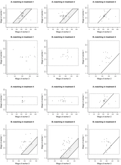
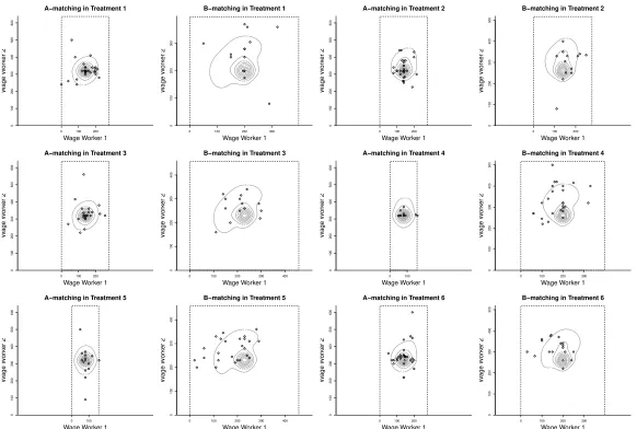
Figure 1: The experimental data in relation to the core. (Note that if B-matching is

inefficient, then the core predictsA-matching, and vice versa.)

0 100 200 300 400 500 600

0

100

200

300

A−matching in treatment 1

Wage of worker 2

W

age of w

or

k

er 1

0 100 200 300 400

0

100

200

300

400

B−matching in treatment 1

Wage of worker 2

W

age of w

or

k

er 1

0 100 200 300 400 500 600

0

100

200

300

Wage of worker 2

W

age of w

or

k

er 1

0 100 200 300 400 500

−100 0 100 200 300 400

Wage of worker 2

W

age of w

or

k

er 1

0 100 200 300 400 500 600

0

100

200

300

Wage of worker 2

W

age of w

or

k

er 1

0 100 200 300 400

0

100

200

300

400

Wage of worker 2

W

age of w

or

k

er 1

0 100 200 300 400 500 600

−100

0

100

200

300

Wage of worker 2

W

age of w

or

k

er 1

0 100 200 300 400 500

0

100

200

300

400

Wage of worker 2

W

age of w

or

k

er 1

0 100 200 300 400 500 600

−100

0

100

200

300

Wage of worker 2

W

age of w

or

k

er 1

0 100 200 300 400

0

100

200

300

400

Wage of worker 2

W

age of w

or

k

er 1

0 100 200 300 400 500 600

0

100

200

300

Wage of worker 2

W

age of w

or

k

er 1

0 100 200 300 400 500

0

100

200

300

400

Wage of worker 2

W

age of w

or

k

(8)

Table 1: Productivities of matches in the six experimental treatments

T1 T2 T3 T4 T5 T6

C1,1 C1,2

C2,1 C2,2

280 400 400 640

280 280 520 640

280 460 460 640

160 400 520 640

160 460 460 640

280 400 520 640

Note: Cw,f is the productivity of the match(w,f)∈W×F. The pairings in the socially efficient

matching are underlined if unique. InT3 andT6, both matchings are efficient.

Experimental logistics, instructions, and basic descriptive statistics are discussed

in Otto and Bolle (2011) and reviewed in the supplementary material.4 _The

observa-tions that are most relevant for our purpose are summarized in Figure 1. It plots all outcomes in relation to the core in the various treatments and illustrates the main styl-ized facts mentioned above (see also Tenbrunsel et al., 1999). The core predicts poorly, overall less than 20% of the observations are in the core, inefficient matching can be observed regularly, and overall observations are more egalitarian than predicted by the

core.5 Two possible explanations for these systematic observations are that subjects

have social preferences and that the stability requirements of the core are too strong or computationally too complex. This possible sources are investigated in the next section.

3 Interdependent preferences or limited depth of

rea-soning?

In this section, we introduce the three basic core concepts for players with interde-pendent preferences based on which we seek to understand whether limited depth of reasoning or interdependence of preferences is responsible for the biases observed in

Figure 1. We consider preferences that are interdependent in the sense thati’s utility

may depend on all of the entities that he can explicitly observe in the experiment: the

4_{Briefly, the order of the treatments and the individual allocation to positions was randomized over}

the sessions. Every subject was allocated to a worker position three times and to a firm position three times. No subject interacted with the same co-participant in more than three of the six games. As Otto and Bolle (2011) verified, there was no indication of reputation building or learning.

5_{In addition, incomplete matching has been observed in 12% of the games. As Otto and Bolle}

(2011) verified, almost all of these incompletions result from last-second rematching of the provisional partners, i.e. just before the 10-minute time line for the negotiations ended. These incomplete matches are therefore not intended by the unmatched players and as such unexplainable by concepts such as the core. In our analysis, we therefore discard these 12% of the observations.

(9)

own payoff, the partner’s payoff, and the partner’s identity. This requires additional

notation. The set of players is N =W ∪F, and the set of i’s potential partners is

Ni=F∪ {/0}ifi∈W andNi=W∪ {/0}ifi∈F (“/0” indicates thatiremains single).

The utility ofi∈N is a functionUi(xi,xj,j):R2+×Ni→R.

In order to define the core for such generalized utilities, we have to account for two new phenomena. On the one hand, the stability of an outcome depends on the matching that applies, since utilities depend on the matching. Hence, the definition of “outcome” needs to be extended to also include the matching. Define a matching

mas a function m:N →N∪ {/0}satisfying, for alli∈N,m(i)∈Ni andm(i)6= /0⇒

m(m(i)) =i. LetMbe the set of all these matchings. The set of outcomes can now be

defined as

X=

(x,m)∈RN+×M| ∀i∈N:m(i) = /0⇒xi=0 and

∀w∈W : m(w)6= /0⇒xw+xm(w)≤Cw,m(w) .

On the other hand, when defining stability under generalized utilities, we need to explicitly take into account that it may be preferable to be single than to share the surplus generated by a match in a highly asymmetric way. Being single will usually

not be stable, but it has to be included as an option. To this end, letCw,/0=C/0,f =0

for allw,f denote the productivity of single players, and letU/0 =0 denote the utility

of the dummy player “/0” who represents the partner of an unmatched player.

Definition 3.1 (Core). The core is the set of outcomes (x,m)∈Xsuch that, for all

i∈N, all j∈Ni, and allx′∈[0,Ci,j],

Ui(xi,xm(i),m(i))≥Ui(x′,Ci,j−x′,j) or Uj(xj,xm(j),m(j))≥Uj(Ci,j−x′,x′,i).

The literature following Selten (1972) has analyzed a solution concept that weak-ens the stability requirements of the core. Selten’s equal-division core, to which we

will refer aslevel-2 core, states that an outcome is stable whenever no pair of players

exists who would benefit if they coalesce and share their surplus equally. Thus, the players consider only a specific alternative outcome rather than all possible alterna-tives.

(10)

that, for alli∈N, all j∈Ni, andx′=Ci,j/2,

Ui(xi,xm(i),m(i))≥Ui(x′,Ci,j−x′,j) or Uj(xj,xm(j),m(j))≥Uj(Ci,j−x′,x′,i).

Otto and Bolle (2011) reduce the rationality requirement even further and say that an outcome may already be stable if the allocations are sufficiently close to the

equal split in all matches. This level-1 corereflects the idea that players may not try

to predict possible payoff allocations in alternative matches at all, arguably due to the uncertainty underlying the necessary negotiations.

Definition 3.3 (Level-1 core). Fix γ >0. The level-1 core is the set of outcomes

(x,m)∈Xsuch that for alli∈N,Ui(xi,xm(i),m(i))≥Ui(Ci,m(i)/2,Ci,m(i)/2,m(i))−γ.

The level-1 core turned out to be most descriptive concept in Otto and Bolle (2011). Two potential objections to this result are that Otto and Bolle’s analysis ne-glected interdependent preferences, while higher-level cores may be more descriptive if we account for those, and that their result may possibly not be robust to changing circumstances. In order to examine robustness, we will distinguish descriptive and

predictive adequacy. The descriptive adequacy is determined by fitting the

parame-ters to the whole sample and evaluating their fit on this very sample. The predictive

adequacyis determined by fitting the parameters to the observations from four of the

six treatments, evaluating their fit on the observations from the remaining two treat-ments, and rotating so that all observations are used exactly once in the evaluation

stage once.6

Since we are also interested in verifying whether the results obtained by maxi-mizing the likelihood of the logit core, as done below, differ qualitatively from those

obtained by maximizing Selten’s score7_{for the core (as proposed in the literature), we}

6_{This approach combines cross validation (Burman, 1989; Zhang, 1993) with non-random holdout}

samples (Keane and Wolpin, 2007). Exploring predictive adequacy as a measure of robustness has been advocated recently by Hey et al. (2010) and Wilcox (2008, 2011), amongst others.

7_{The “Selten score” (Selten, 1972, 1991) measures the goodness of fit in this case where likelihoods}

are not available (they are zero whenever a single observation is not in the core), and where sums of squared differences are not available as there is not reliable measure for the distance between A

-matching andB-matching.Selten’s scoreof a solution concept is the difference between (i) the relative

frequency of observations compatible with the concept and (ii) the share of internally Pareto efficient outcomes compatible with the concept. An outcome(x,m)∈Xis “internally Pareto efficient” if the

players allocate the whole surplus generated within their matches, i.e. ifm(i)6=/0andxi+xm(i)=Ci,m(i)

for alli∈N.

(11)

[image:11.595.105.486.143.216.2]

Table 2: Selten scores (higher is better) for egoistic and altruistic preferences

# Parameters Descriptive adequacy Predictive adequacy

Ego Altr Egoism Altruism Egoism Altruism

Level-1 Core 1 3 0.575 0.612 0.574 0.586

Level-2 Core 0 2 0.312 0.512 0.312 0.509

Core 0 2 0.122 0.276 0.122 0.253

Note: Level-1 core, level-2 core, and core are defined in Definitions 3.1–3.3; the Selten score

is defined in Footnote 7.

now evaluate the three core variants in terms of Selten’s score, allowing for egoistic

and altruistic interdependent preferences.8 The altruistic utility function is defined as

Ui(xi,xj,j) =xi+αxj+βCi j, where αand βare free parameters andCi j is the

pro-ductivity (i.e. sum of payoffs) in the other match. In case i is single, i.e. j= /0, the

utility isUi(0,0,/0) =0+β·max{C2,1,C2,2}. The model parameters are estimated by

maximizing Selten’s score jointly over all parameters, using a gradient free algorithm for the initial approach to the maximum, a Newton method to ensure convergence, and various starting values to verify globality of the maximum.

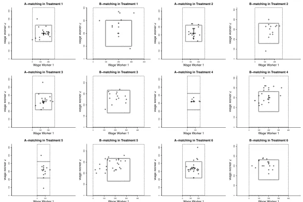
The results are summarized in Table 2. The best fitting concepts are the level-1 core with either egoistic or altruistic preferences and the level-2 core for altruistic preferences. They each contain approximately 80% of the observations but cover only 20%–30% of the outcome space. Their Selten scores do not differ significantly (in

Wilcoxon-tests of Selten’s scores at the session level, with p=.02) and they all fit

significantly better than all other models (at p< .001). Thus, the bias of the core

ob-served in Figure 1 appears to be primarily due to the limited level of reasoning, i.e. the limited grasp of possible outcomes in alternative matches, while interdependent preferences seem to be of minor relevance at best. Further, as the predictive adequacy reported in Table 2 and the plot in Figure 2 show, the prediction bias is robustly elim-inated in the level-1 core. In the remaining two sections, we introduce and analyze random utility cores, in order to account for the fact that the observations are not dis-tributed uniformly on the level-1 core, that the incompatible ones do not seem to be uniformly outside of it, and that observations outside of the core occur in the first place. This will allow us to extract all information contained in the data set and make likelihood-based inference.

8_{Further analysis, which is provided in the supplementary material, shows that inequity aversion}

(12)

[image:12.842.107.719.102.510.2]

Figure 2: The level-1 core of players with egoistic preferences (withγ=100 in all cases)

Wage Worker 1

W

age W

or

k

er 2

0.1 0.2 0.3 0.4 0.5

0.6 0.7 0.8 0.9 1

0 100 200

0 100 200 300 400 500 600

A−matching in Treatment 1

Wage Worker 1

W

age W

or

k

er 2

0.1 0.2 0.3 0.4 0.5 0.6

0.7 0.8 0.9

1

0 100 200 300 400

0

100

200

300

400

B−matching in Treatment 1

Wage Worker 1

W

age W

or

k

er 2

0.1 0.2 0.3 0.4 0.5

0.6 0.7 0.8 0.9 1

0 100 200

0 100 200 300 400 500 600

Wage Worker 1

W

age W

or

k

er 2

0.1 0.2 0.3 0.4 0.5

0.6 0.7 0.8 0.9

1

0 100 200

0 100 200 300 400 500

Wage Worker 1

W

age W

or

k

er 2 0.1 0.2 0.3 0.4 0.5

0.6 0.7 0.8 0.9 1

0 100 200

0 100 200 300 400 500 600

Wage Worker 1

W

age W

or

k

er 2

0.1 0.2 0.3 0.4 0.5 0.6

0.7 0.8 0.9

1

0 100 200 300 400

0

100

200

300

400

Wage Worker 1

W age W or k er 2 0.1 0.1 0.2 0.2 0.3 0.3 0.4 0.4 0 100 0 100 200 300 400 500 600

Wage Worker 1

W

age W

or

k

er 2

0.1 0.2 0.3 0.4 0.5

0.6 0.7 0.8 0.9

1

0 100 200 300 400

0 100 200 300 400 500

Wage Worker 1

W age W or k er 2 0.1 0.1 0.2 0.2 0.3 0.3 0.4 0.4 0 100 0 100 200 300 400 500 600

Wage Worker 1

W

age W

or

k

er 2

0.1 0.2 0.3 0.4 0.5 0.6

0.7 0.8 0.9

1

0 100 200 300 400

0

100

200

300

400

Wage Worker 1

W

age W

or

k

er 2 0.1 0.2 0.3 0.4 0.5

0.6 0.7 0.8 0.9 1

0 100 200

0 100 200 300 400 500 600

Wage Worker 1

W

age W

or

k

er 2

0.1 0.2 0.3 0.4 0.5

0.6 0.7 0.8 0.9

1

0 100 200 300 400

0 100 200 300 400 500

(13)

4 Explaining the outcome distribution: The logit core

Simple bargaining games

Initially, consider a simple bargaining problem. There are two players negotiating the

allocation of a cake valuedC>0. We define the random utility bargaining problem by

adding a random utility component to the outside option. The distribution of the ran-dom component is general in the following definition, but it will be logistic in all sub-sequent applications, i.e. the difference of two i.i.d. extreme-value distributed random variables. This corresponds closely with the approach taken in non-cooperative game theory (see e.g. McKelvey and Palfrey, 1995, Goeree and Holt, 1999, Weizsäcker, 2003, Turocy, 2005). Illustrations follow shortly.

Definition 4.1 (Random utility bargaining game). The set of players is N ={1,2},

the set of possible outcomes isX={x∈R2+|x1+x2≤C}for someC>0, and the

players’ disagreement payoffs are x₁,x₂∈[0,C] with x₁+x₂ <C. For both i∈N,

utilities are ui(x) =xi for all x∈X and ˜ui(x) =xi+εi for the outside option. The

distributions ofε1andε2are continuous, stochastically independent, and characterized

by the cumulative distribution functionsF1andF2, respectively.

In the unperturbed game, an allocation is “stable” if and only if it is individually

rational and Pareto efficient. The coreXc⊆Xis the set of stable allocations.

XC=

x∈X|xi≥xi ∧ xj≥xj ∧ xi+xj=C

If utilities are random, stability becomes a stochastic property, as individual rationality

is stochastic. The probability that playeriis content withxis Pr(xi≥xi+εi), and the

probability thatxis individually rational (i.e. that both players are content) is

π(x) =Pr(xi≥xi+εi)·Pr(xj≥xj+εj). (1)

This probability is called the stochastic stability of x, and an outcome x is called

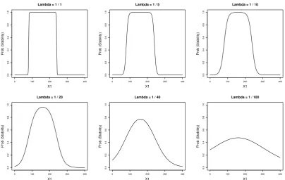
stochastically more stable than x′ if π(x)>π(x′). Figure 3 plots the probabilities

that outcome(x1,x2)is individually rational conditional on Pareto efficiency (i.e.x2=

C−x1), assuming logistic perturbations. If the utility perturbations εi have logistic

distribution with scale parameter s=1/λ, then i is content with probability 1/

(14)

[image:14.595.90.495.146.402.2]

Figure 3: Stochastic stability in bargaining games for varying precisionsλ

0 100 200 300 400

0.0 0.2 0.4 0.6 0.8 1.0

Lambda = 1 / 1

X1

Prob (Stability)

0 100 200 300 400

0.0 0.2 0.4 0.6 0.8 1.0

Lambda = 1 / 5

X1

Prob (Stability)

0 100 200 300 400

0.0 0.2 0.4 0.6 0.8 1.0

Lambda = 1 / 10

X1

Prob (Stability)

0 100 200 300 400

0.0 0.2 0.4 0.6 0.8 1.0

Lambda = 1 / 20

X1

Prob (Stability)

0 100 200 300 400

0.0 0.2 0.4 0.6 0.8 1.0

Lambda = 1 / 40

X1

Prob (Stability)

0 100 200 300 400

0.0 0.2 0.4 0.6 0.8 1.0

Lambda = 1 / 100

X1

Prob (Stability)

Note:The cake size isC=400 and the outside options are x₁,x₂

= (120,240). The plotted functions are Pr(x1≥x1+ε1andx2≥x2+ε2),ε1,ε2being i.i.d. logistic, as functions ofx1withx2=C−x1.

exp(λ(x_i−xi)).

This ordering of outcomes generalizes deterministic stability in an intuitive way.

As the precision λ tends to infinity, stochastic stability converges pointwise to the

stability indicator 1_x∈XC of the unperturbed game. The stochastically most stable

allocation is generally in the interior of the core of the unperturbed game, and if perturbations are identically distributed for the players, the stochastically most sta-ble outcome is the Nash solution. This is easy to see if perturbations are logistic

Fi(r) =1/ 1+exp(−λir)

for allr∈Randi∈N. In this case, the stochastic stability

π(x) = 1+e−λi(xi−xi)−1∗ 1+_e−λj(1−xi−xj)−1is maximized if

1+eλi(xi−xi)

1+eλj(1−xi−xj) =

λi

λj

.

If errors are i.i.d. logistic, then λi=λj and the most stable outcome is the Nash

bar-gaining solution. The following result establishes equivalence between the Nash solu-tion and the stochastically most stable outcome for a general class of distribusolu-tions.

(15)

Lemma 4.2. Assume the random utility components of all players are i.i.d. with

cumu-lative density F. If F is symmetric, F(x) =1−F(−x), and has quasi-concave density,

then the unique maximizer ofπ(x)is xi= (xi+C−xj)/2and xj= (xj+C−xi)/2.

Proof. The first-order condition for maxxiF(xi−xi)∗F(C−xi−xj)yields

f(xi−xi)/f(C−xi−xj) =F(xi−xi)/F(C−xi−xj).

The claimed solution impliesxi−xi=C−xi−xj=:x′and hence satisfies the

condi-tion. Next, x_i+x_j<Cimpliesx′= (C−x_i−x_j)/2>0. The second-order condition

(for the claimed solution to be a maximum) is 2f′(x′)F(x′)<2f(x′)f(x′). By

sym-metry and quasi-concavity, x′>0 implies f′(x′)≤0; since all other terms are

pos-itive, the condition holds. Finally, consider the case xi−xi6=x′, and without loss,

assume xi−xi >x′. Hence, C−xi−xj < x′. By symmetry and quasi-concavity,

f(xi−xi)≤ f(C−xi−xj), and by monotonicity,F(xi−xi)>F(C−xi−xj); hence,

the first-order condition is violated, which proves uniqueness.

Further, outcomes close to the Nash solution are stochastically more stable than distant outcomes, outcomes in the core are stochastically more stable than outcomes outside of it, and outcomes close to the core are stochastically more stable than out-comes distant to the core. These characteristics correspond closely with the intuition that we wish to capture, and for this reason we define a solution concept where the

probability that outcome x results is proportional to its stochastic stability.

Specifi-cally, the random utility coreis the probability density fC ∈∆ PF(X)

on the Pareto frontier that is proportional to the above measure of stochastic stability.

fC(x) =π(x)/ Z

PF(X)π x˜

dx˜ (2)

As stated, the integration is along the Pareto frontier defined as PF(X) ={x∈X|x≥

x′ ∀x′ ∈X}. Obviously, Pareto efficiency could be relaxed as well, similar to the

(16)

Proposition 4.3. For bargaining games (Def. 4.1), the following statements are

equiv-alent.

1. fCsatisfies Eq.(2)forπ(x) =F1(x1−x1)∗F2(x2−x2).

2. fCsatisfies the following conditions.

A1 Continuity and Pareto efficiency: fC is the density of a continuous

distri-bution on PF(X).

A2 Proportional stability: fC(x) is proportional to the probability that all

players preferxto their outside option, i.e. toPr ui(x)≥u˜i(x)∀i

.

Proof. 2.⇒1.: By the definition of the game, ε1 and ε2 are independent, and thus

Pr ui(x)≥u˜i(x) ∀i

=Pr u1(x)≥u˜1(x)·Pr u2(x)≥u˜2(x)=:π(x). A2 implies

fC(x) =a·π(x)for somea>0. Finally, since fC is a density with support only on the

Pareto frontier (A1),a=1/R_PF₍_X₎π(x)dx. 1.⇒2.can be verified easily.

Note that A2 implies independence of irrelevant alternatives (IIA), i.e. fC(x′|X′)·

fC(x|X′′) = fC(x′|X′′)·fC(x|X′)for allx,x′∈X′and all measurableX′⊆X′′⊆PF(X).

Assignment games

Assignment games generalize bargaining games by endogenizing the outside options. For each player, every feasible partner other than his current one represents an outside option, while the values of these outside options depend on the payoff allocations negotiated in their matches. The more my prospective partners in their current matches make, the less the outside options are worth to me. Aside from taking these changes into account, the above definition of the random utility core generalizes immediately. In particular, we maintain the assumption that the utilities of the outside options are random (e.g. logistic in the logit core).

Definition 4.4(Random utility assignment game). For each outcome(x,m)∈X, the

utility of i∈N is ui(x,m) =Ui(xi,xm(i),m(i)). The utility of the blocking coalition

(i,j), j6=m(i), with wages (xi,xj)∈R2+ is ˜ui(xi,j) =Ui(xi,xj,j) +εi,j, and the

util-ity of the outside option is ui(xi,/0) =Ui(0,0,/0) +εi,/0. The distributions of εi,j are

continuous and stochastically independent over alli∈N and j∈Ni.

(17)

As before, we define stochastic stability as the probability that the allocation is stable, i.e. that no pair of players can rematch profitably. In the random utility

assign-ment game, the stochastic stability of outcome(x,m)therefore is

π(x,m) =Pr ∀i∈N,∀j∈Ni,∀x′∈[0,Ci,j]:

ui(x,m)≥u˜i(x′,j)oruj(x,m)≥u˜j(Ci,j−x′,i), (3)

and exploiting all independence assumptions in Def. 4.4, it simplifies to

π(x,m) =

_∏

i∈Nj

∏

∈Ni

Z

R

Z

R

fi,j(εi,j)fj,i(εj,i)1

∀x′∈[0,Ci,j]:

Ui(xi,xm(i),m(i))≥Ui(x′,Ci,j−x′,j) +εi,jor

Ui(xj,xm(j),m(j))≥Uj(Ci,j−x′,x′,i) +εj,i dεi,jdεj,i. (4)

Intuitively, at the beginning of the assignment game, the utility perturbations (εi,j)

are drawn. One may think of εi,j as a measure of the “chemistry” between i and j

(in the eyes of i). The players then play the assignment game and evaluate possible

allocations by comparing them to the outside options plus the utility perturbations. The stochastic stability is the ex-ante probability that a given allocation will be stable.

The random utility core is again defined as the density of continuous distribution on the Pareto frontier. We assume that players are able to match completely and to

allocate the whole surplus generated in their respective match.9 Let IPF(X′) denote

the set of such allocations withinX′⊆Xand letM∗⊂Mdenote the set of complete

matchings. Now, usingXm={x∈Rn|(x,m)∈X}, the random utility core is

fC(x,m) =π(x,m)/

∑

m∈M∗

Z

IPF(Xm)

π x˜,mdx˜. (5)

Clearly, the random utility core converges pointwise to the uniform distribution on the core if the utility variances approach zero. The assumption that stochastic stability and outcome density are proportional is particularly simple and it turns out to fit our data well (see below). Alternative assumptions may prove appropriate in alternative

9_{That is, we assume that outcomes satisfy internal Pareto efficiency as defined in Fn. 7. These}

(18)

classes of games.

Proposition 4.5. For any assignment game, the following statements are equivalent.

1. fCis the random utility core defined in Eqs.(3)and(5).

2. fCsatisfies the following conditions.

A1 Continuity and internal Pareto efficiency: fCis the density of a continuous

distribution on the set outcomes satisfying internal Pareto efficiency.

A2 Proportional stability: fC(x,m)is proportional to the stochastic stability

π(x,m).

Proof. The proof is very similar to that of Prop. 4.3 and therefore skipped.

Finally, the stochastic stabilities of level-1 and level-2 cores follow straightfor-wardly. The level-1 core with random utility has the stochastic stability

π(x,m) =Pr ∀i∈N: ui(x,m)>u˜i(Ci,m(i)/2,m(i))

, (6)

and the level-2 core has the stochastic stability

π(x,m) =Pr ∀i∈N,∀j∈Ni,x′=Ci,j/2 :

˜

ui(x′,j)≤ui(x,m)or ˜uj(Ci,j−x′,j)≤uj(x,m). (7)

5 Econometric evaluation of the logit core

In this section, we evaluate both descriptive and predictive adequacy of the logit core revisiting the data of Otto and Bolle (2011). As above, descriptive adequacy measures the goodness of fit to the whole sample after fitting the parameters to the whole sam-ple, and predictive adequacy measures the goodness of fit out of samsam-ple, after fitting parameters to a subset of treatments, evaluating the predictions on the remaining treat-ments, and rotating such that all treatments are used once. We consider the logit core in all three variants (level-1 core, level-2 core, core) and contrast it with regression models and random behavior cores for further robustness checking. In all cases, the likelihood is maximized jointly over all parameters by first gradient-free and second

(19)

Newton methods, and a variety of starting values is used to verify globality of the max-imum. Table 3 lists absolute values of the log-likelihoods for all models and Figure 4

illustrates the fit of the best-fitting model.10

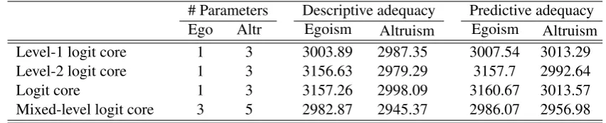
As for the logit cores, see Table 3a, the level-1 core for egoistic preferences and

the level-2 core for altruistic preferences do not differ significantly (p>0.1) and the

latter fits significantly better than all other concepts (p<0.1).11 The difference

be-tween descriptive and predictive adequacy is insignificant for these concepts, i.e. the result is robust and not due to overfitting. This confirms that subjects do not consider all possible outcomes in alternative matches when they evaluate their current situation. The observation that level-1 and level-2 cores fit the data similarly well is surprising, however. The experiment had been designed to distinguish explicitly between these possibilities. In all treatments, we can distinguish “strong” and “weak” players, based on payoffs from their respective outside options (the alternative match). Thus, either the alternative match is strategically relevant, in which case the level-2 core should fit better than the level-1 core, or income equality is of primary relevance, in which case the level-1 core should fit better. Since both concepts fit similarly, we infer that indeed

both motives are of strategic relevance and affect “stability” of outcomes.12

In order to investigate this hypothesis more conclusively, consider the following

mixed-level corenesting both level-1 and level-2 cores. Its stochastic stability index is

the weighted mean of the stochastic stabilitiesπ₁in the level-1 logit core for egoistic

preferences and π2 in the level-2 logit core for altruistic preferences (which are the

best-fitting concepts out of sample), with weightsµ∈[0,1].

πmix(x,m) = (1−µ)·π1(x,m) +µ·π2(x,m) (8)

The level-1 core obtains forµ=0, the level-2 core obtains forµ=1, and other values

ofµyield mixtures of these concepts. Table 3b reports the parameter estimates and

Ta-10_{The supplementary material contains all parameter estimates, the results of likelihood-ratio tests}

(nested and non-nested Vuong tests) conducted to verify significance of differences in goodness of fit, and analyses of alternative models with (amongst others) inequity averse players.

11_{The Vuong (1989) tests for nested/nested models (as appropriate) are done using}

non-parametric tests at the session level. That is, with(fs)28_s₌1and(gs)28s=1denoting the log-likelihoods of

two competing models in the 28 independent sessions, we evaluate the null hypothesisH0: ln(fi/gi) =0

using Wilcoxon signed-rank tests. All test results are provided as supplementary material.

12_{Note that this is not a matter of social preferences, as we explicitly tested for inequity aversion, as}

(20)

[image:20.595.89.515.159.246.2]

Table 3: Goodness of fit: Overview of all models

(a) Goodness-of-fit|LL|of the random utility (logit) cores

Level-1 logit core 1 3 3003.89 2987.35 3007.54 3013.29

Level-2 logit core 1 3 3156.63 2979.29 3157.7 2992.64

Logit core 1 3 3157.26 2998.09 3160.67 3013.57

Mixed-level logit core 3 5 2982.87 2945.37 2986.07 2956.98

(b) Parameter estimates of the mixed-level logit core with altruism

λ1 λ2 α β µ LL

13.5567

(1.4161) 32(3..62588933) −(00..053489)

−0.2537

(0.0537)

0.0294

(0.0084) −2945.37

Note:λ1andλ2are the precision parameters of the level-1 and level-2 components (resp.) of the

mixed core defined in Eq. (8),α,βare the altruism coefficients, andµis the mixture weight. The

standard errors are obtained from the information matrix.

(c) Goodness-of-fit|LL|of the random behavior cores

Level-1 core 1 3 3085.07 3057.39 3085.70 3068.21

Level-2 core 1 3 3225.18 3106.25 3225.79 3330.29

Core 1 3 3253.32 3191.34 3255.17 3208.04

(d) Goodness-of-fit of the regression models

#Pars Descriptive|LL| Predictive|LL|

Regression on treatment parameters

Restricted coefficients 14 2971.60 3052.92

Unrestricted coefficients 24 2964.04 3038.54

Regression on theoretically relevant parameters

Restricted coefficients 7 3006.40 3015.56

Unrestricted coefficients 11 2979.82 3120.54

Note: The “treatment parameters” are the three productivities C1,1, C1,2, C2,1 that are not

con-stant across treatments, and the “theoretically relevant parameters” are the efficiency difference be-tweenA- andB-matching, i.e. the difference(C1,1+C2,2)−(C1,2+C2,1)and the symmetric

indica-torIC1,2=C2,1. In the models with “restricted coefficients”, the regression coefficients are equal across

A andB matching, in those with “unrestricted coefficients”, this restriction is lifted. For example,

under the “Regression on treatment parameters” model, the probability of A-matching is Pr(A) =

1/ 1+exp(−I0−p0,C1,1C1,1−p0,C1,2C1,2−p0,C2,1C2,1)

_{, wages of workers}

i∈ {1,2} are distributed as f(wi) =Pr(A)·f(wi|A) + (1−Pr(A))·f(wi|B), withwi|M∼N Ii|M+pi|M,C1,1C1,1+pi|M,C1,2C1,2+

pi|M,C2,1 C2,1,σ2i|M

and support

0,wi|M

, using (w1|A,w2|A,w1|B,w2|B) = (C1,1,C2,2,C1,2,C2,1). The

other models are defined correspondingly (details are provided in the supplementary material).

(21)

[image:21.842.126.708.145.537.2]

Figure 4: Contour plots of the relative stochastic stabilities for the mixed-level logit core with altruistic preferences. The iso-lines connect outcomes with the same stochastic stability and hence the same predicted density. Outcomes along the the outmost line (at “0.1”) have 10% of the stochastic stability (and density) of the stochastically most stable outcome in the respective game.

Wage Worker 1

W age W or k er 2 0.1 0.2 0.3 0.4 0.5

0 100 200

0 100 200 300 400 500 600

Wage Worker 1

W age W or k er 2 0.1 0.2 0.3 0.4 0.5 0.6

0 100 200 300

0

100

200

300

Wage Worker 1

W age W or k er 2 0.1 0.2 0.3 0.4 0.5

0 100 200

0 100 200 300 400 500 600

Wage Worker 1

W age W or k er 2 0.1 0.2 0.3 0.4 0.5

0 100 200

0 100 200 300 400 500

Wage Worker 1

W age W or k er 2 0.1 0.2 0.3

0.4 0.5

0 100 200

0 100 200 300 400 500 600

Wage Worker 1

W age W or k er 2 0.1 0.2 0.3 0.4 0.5

0 100 200 300 400

0

100

200

300

400

Wage Worker 1

W

age W

or

k

er 2 0.1

0.2 0.3 0.4 0.5 0 100 0 100 200 300 400 500 600

Wage Worker 1

W age W or k er 2 0.1 0.2 0.3 0.4 0.5

0 100 200 300

0 100 200 300 400 500

W age W or k er 2 0.1 0.2 0.3 0.4 0.5 100 200 300 400 500 600

W age W or k er 2 0.1 0.2 0.3 0.4 0.5 100 200 300 400

W age W or k er 2 0.1 0.2 0.3 0.4 0.5 100 200 300 400 500 600

W

age W

or

k

er 2

0.1 0.2

0.3 0.4 0.5 100 200 300 400 500

(22)

ble 3a reports descriptive and predictive adequacy. It shows that the mixed-level core allowing for interdependent preferences (i.e. spite) improves the goodness of fit sub-stantially, by at least 30 log-likelihood points in relation to all other models, and as we

verified in Vuong tests, these differences are highly significant (p< .01) in all cases.

Although the spite coefficients are highly significant, too, even the mixed-level core with egoistic preferences improves on all other models. We therefore conclude that the subjects’ main criterion for stability is equality of incomes within matches, while the potential payoff from the alternative match and the interdependence of preferences are of secondary, but significant relevance.

Comparing these results with those obtained by maximizing the Selten score in Section 3, two observations are noteworthy. On the one hand, the mixed-level core, which is the unambiguously best-fitting model here, cannot be defined without intro-ducing the notion of stochastic stability. Thus, the logit core substantially extends the range of models that can be considered. On the other hand, between the models considered above, the ranking of the three best models actually inverted, toward (1) Level-2 Altruism, (2) Level-1 Egoism, and (3) Level-1 Altruism, with the difference between (1) and (3) even being significant. This follows from using all information contained in the distribution of outcomes, such as the distance from an outside ob-servation to the core, and in particular by smoothening the transition between close misses and close hits. In addition, of course, the maximum likelihood estimates allow for straightforward computation of standard errors as well as model evaluation based on likelihood-ratio tests and information criteria.

Figure 4 shows that the mixed-level core also fits qualitatively. Its Cox-Snell

pseudo-R2 is ˜R2 = 0.9239,13 which confirms the positive visual impression of the

plots. The estimated utility parameters are α =−0.49 and β=−0.25 (Table 3b),

which confirms that players are spiteful when evaluating alternative outcomes. This indicates competitive bargaining and thus seems to be reasonable.

Finally, we conduct two robustness checks to verify the results. On the one hand, the logit core was defined to capture the distribution of the observations inside the core, as central observations are more frequent than borderline observations, as well as the distribution outside the core, as borderline observations are more frequent than

13_{The Cox-Snell pseudo-}_R2 _{is ˜}_R2₌₁₋₍_L₍_Baseline₎_/_L₍_Model₎₎2/N _with_L _{being the likelihood}

function and the Baseline model being the model predicting uniform randomization. Its log-likelihood is−3276.27 and the number of observations isN=257.

(23)

distant observations. To verify this implication, define arandom behavior core with

uniform noise as follows: Outcomes are distributed either uniformly inside the core,

with probability 1/(1+ε), or uniformly outside the core, with probabilityε/(1+ε).

As ε tends to zero, this random behavior core converges uniformly to the uniform

distribution on the core, as does the logit core as noise disappears, and it has the same number of parameters. The only difference is the specification of noise. Its definition applies to level-1 and level-2 cores straightforwardly. Table 3c reports the descriptive and predictive adequacy of all six (basic) variants. It shows that random behavior cores fit uniformly worse than their respective logit core counterparts, and all of these

differences are highly significant. In addition to Figure 4 and pseudo-R2 reported

above, this confirms that the continuous stochastic stability implied by the logit core fits the outcome distribution well.

On the other hand, the core is a strategic model, and to verify whether this is a fruitful approach toward analyzing negotiation outcomes in the first place, let us now examine non-strategic and reduced-form regression models. As shown above, subjects evaluate outcomes primarily by their difference to the equal split, which suggests that regression models may fit indeed. We investigate this hypothesis on four alternative regression models, in order to be able to address this issue conclusively. Similarly

to the logit cores, all regression models must predict the probabilities of A and B

matching as well as the distribution of wagesw1,w2. The first two models are standard

and regress these variables on the treatment parametersC1,1,C1,2,C2,1(note thatC2,2

is held constant in all treatments). The other two models represent the prediction of the best fitting structural model, the mixed-level core, in reduced form. They use the

same information, namely the efficiency gain in A-matching, the symmetry indicator

IC₁,2=C2,1, and the values of the outside options in each form of matching. For each

class of models, we distinguish a parsimonious “restricted” form, where the wage

coefficients are constant across AandBmatching, and an “unrestricted” form where

coefficients are flexible (for further information, see the note to Table 3d).

The goodness-of-fit measures for all models are listed in Table 3d. Three of the

four regression models improve upon the level-klogit cores in-sample, which confirms

that the basic distribution can be fit using regression. However, these three models overfit drastically and their predictive adequacy is poor—they are significantly worse

thanallrandom utility models allowing for altruistic preferences. Thus, the in-sample

(24)

not allow for reliable inference. The single regression model that avoids overfitting is the regression on “strategically relevant parameters” with “restricted coefficients”, which has poor descriptive and predictive adequacy, however. Thus, we conclude that the strategic solution concept “logit core” is substantially more adequate in predicting (laboratory) assignment outcomes than at least such “standard” regression models.

6 Conclusion

This paper has analyzed cooperative assignment games with the intention of under-standing the sources of the prediction bias implied by the core. The competing hy-potheses were that subjects have interdependent preferences or limited depth of rea-soning. In order to fully capture the distribution of observations, and to extract all information contained therein, we extended the core concept to allow for random util-ity perturbations—an approach that proved descriptive in many previous experiments on decision theory and non-cooperative game theory. We found that the logit core in-deed fits the distribution of outcomes and that subjects deviate from the core primarily due to a severely limited grasp (or due to severe discounting) of possible outcomes in alternative matches. Stable outcomes tend to be close to the equal split, as the “level-1 core” is the main component of the identified model, while alternative matches tend to matter only under the simplified assumption that the equal split will obtain there, and interdependence of preferences is significant but of minor relevance. The identi-fied model nests level-1 and level-2 cores and fits both qualitatively and quantitatively, notably without overfitting.

Both interdependence of preferences and random utility perturbations are novel in analyses of cooperative games. Their adequacy in the present analysis and their widespread use in non-cooperative game theory suggest that further research is war-ranted. Besides further analyses of random-utility concepts in cooperative bargaining games, further research may also investigate values of games with random utility, and perhaps most interestingly, it may evaluate the descriptive and predictive adequacies of cooperative and non-cooperative models in comparative studies. This may help to map out their respective fields of application and to define new concepts modeling the key insights from both branches.

(25)

References

Berl, J., McKelvey, R., Ordeshook, P., and Winer, M. (1976). An experimental test

of the core in a simple n-person cooperative nonsidepayment game. Journal of

Conflict Resolution, 20(3):453–479.

Burman, P. (1989). A comparative study of ordinary validation, v-fold

cross-validation and the repeated learning-testing methods. Biometrika, 76(3):503.

Camerer, C. (2003). Behavioral game theory: Experiments in strategic interaction.

Princeton, NJ: Princeton University Press.

Camerer, C., Ho, T., and Chong, J. (2004). A cognitive hierarchy model of games.

Quarterly Journal of Economics, 119(3):861–898.

Chen, Y. and Sönmez, T. (2002). Improving efficiency of on-campus housing: An

experimental study. American Economic Review, 92(5):1669–1686.

Chen, Y. and Sönmez, T. (2006). School choice: an experimental study. Journal of

Economic Theory, 127(1):202–231.

Costa-Gomes, M., Crawford, V., and Iriberri, N. (2009). Comparing models of

strate-gic thinking in Van Huyck, Battalio, and Beil’s coordination games. Journal of the

European Economic Association, 7(2-3):365–376.

Crawford, V. and Knoer, E. (1981). Job matching with heterogeneous firms and work-ers. Econometrica, 49(2):437–50.

Driessen, T. (1998). A note on the inclusion of the kernel in the core of the bilateral

assignment game. International Journal of Game Theory, 27(2):301–303.

Eavey, C. and Miller, G. (1984). Fairness in majority rule games with a core.American

Journal of Political Science, pages 570–586.

Fiorina, M. and Plott, C. (1978). Committee decisions under majority rule: An

exper-imental study. The American Political Science Review, pages 575–598.

Goeree, J. and Holt, C. (1999). Stochastic game theory: for playing games, not just

(26)

Halaburda, H. (2010). Unravelling in two-sided matching markets and similarity of

preferences. Games and Economic Behavior, 69(2):365–393.

Hamers, H., Klijn, F., Solymosi, T., Tijs, S., and Pere Villar, J. (2002). Assignment

games satisfy the coma-property. Games and Economic Behavior, 38(2):231–239.

Hey, J. (1998). An application of Selten’s measure of predictive success.

Mathemati-cal Social Sciences, 35(1):1–15.

Hey, J., Lotito, G., and Maffioletti, A. (2010). The descriptive and predictive adequacy

of theories of decision making under uncertainty/ambiguity. Journal of risk and

uncertainty, 41(2):81–111.

Kagel, J. and Roth, A. (2000). The dynamics of reorganization in matching markets:

A laboratory experiment motivated by a natural experiments. Quarterly Journal of

Economics, 115(1):201–235.

Keane, M. and Wolpin, K. (2007). Exploring the usefulness of a nonrandom holdout

sample for model validation: Welfare effects on female behavior. International

Economic Review, 48(4):1351–1378.

Kelso Jr, A. and Crawford, V. (1982). Job matching, coalition formation, and gross

substitutes. Econometrica, 50(6):1483–1504.

Koopmans, T. and Beckmann, M. (1957). Assignment problems and the location of

economic activities. Econometrica, 25(1):53–76.

McKelvey, R. and Ordeshook, P. (1981). Experiments on the core: Some disconcerting

results for majority rule voting games. Journal of Conflict Resolution, pages 709–

724.

McKelvey, R. and Palfrey, T. (1995). Quantal response equilibria for normal form

games. Games and Economic Behavior, 10(1):6–38.

Nalbantian, H. and Schotter, A. (1995). Matching and efficiency in the baseball

free-agent system: An experimental examination.Journal of Labor Economics, 13(1):1–

31.

Núñez, M. and Rafels, C. (2003). The assignment game: the τ-value. International

Journal of Game Theory, 31(3):411–422.

(27)

Olson, M. and Porter, D. (1994). An experimental examination into the design of decentralized methods to solve the assignment problem with and without money.

Economic Theory, 4(1):11–40.

Otto, P. and Bolle, F. (2011). Matching markets with price bargaining. Experimental

Economics, 14(3):322–348.

Pais, J. and Pintér, Á. (2008). School choice and information: An experimental study

on matching mechanisms. Games and Economic Behavior, 64(1):303–328.

Pérez-Castrillo, D. and Sotomayor, M. (2002). A simple selling and buying procedure.

Journal of Economic Theory, 103(2):461–474.

Quint, T. (1991a). Characterization of cores of assignment games. International

Quint, T. (1991b). The core of an m-sided assignment game. Games and Economic

Behavior, 3(4):487–503.

Quint, T. (1996). On one-sided versus two-sided matching games. Games and

Eco-nomic Behavior, 16(1):124–134.

Roth, A. (1985). Common and conflicting interests in two-sided matching markets.

European Economic Review, 27(1):75–96.

Selten, R. (1972). Equal share analysis of characteristic function experiments. In

Sauermann, H., editor,Contributions to Experimental Economics (Beiträge Zur

Ex-perimentellen Wirtschaftsforschung), pages 130–165. Mohr Siebeck.

Selten, R. (1991). Properties of a measure of predictive success. Mathematical Social

Sciences, 21(2):153–167.

Shapley, L. and Shubik, M. (1972). The assignment game i: The core. International

Solymosi, T. and Raghavan, T. (2001). Assignment games with stable core.

(28)

Sotomayor, M. (1999). The lattice structure of the set of stable outcomes of the

mul-tiple partners assignment game. International Journal of Game Theory, 28(4):567–

583.

Stahl, D. and Wilson, P. (1995). On players’ models of other players: Theory and

experimental evidence. Games and Economic Behavior, 10(1):218–254.

Tenbrunsel, A., Wade-Benzoni, K., Moag, J., and Bazerman, M. (1999). The

ne-gotiation matching process: Relationships and partner selection. Organizational

Behavior and Human Decision Processes, 80(3):252–283.

Toda, M. (2005). Axiomatization of the core of assignment games. Games and

Eco-nomic Behavior, 53(2):248–261.

Turocy, T. (2005). A dynamic homotopy interpretation of the logistic quantal response

equilibrium correspondence. Games and Economic Behavior, 51(2):243–263.

Vuong, Q. (1989). Likelihood ratio tests for model selection and non-nested hypothe-ses. Econometrica, 57(2):307–333.

Weizsäcker, G. (2003). Ignoring the rationality of others: evidence from experimental

normal-form games. Games and Economic Behavior, 44(1):145–171.

Wilcox, N. (2008). Stochastic models for binary discrete choice under risk: A critical

primer and econometric comparison. Risk aversion in experiments, 12:197–292.

Wilcox, N. (2011). Stochastically more risk averse: A contextual theory of stochastic

discrete choice under risk. Journal of Econometrics, 162(1):89–104.

Zhang, P. (1993). Model selection via multifold cross validation. The Annals of

Statistics, 21(1):299–313.