A Study on Multipeutics

(1)

http://www.scirp.org/journal/am ISSN Online: 2152-7393

ISSN Print: 2152-7385

A Study on Multipeutics

Jens Christian Larsen

Vanløse Alle 50 2. mf. tv, 2720 Vanløse, Copenhagen, Denmark

Abstract

Multipeutics is the simultaneous application of m ≥ 4 cancer treatments. m = 4 is quadrapeutics, which was invented by researchers at Rice University, Northeastern University, MD Anderson Cancer Centre and China Medical University, see [1]. Multipeutics is our idea. From section 6 Summary, it fol-lows that multipeutics can be more potent than quadrapeutics by comparing these two mathematical models. The first two treatments in quadrapeutics are systemically administered nano gold particles G and lysosomal chemo thera-peutic drug D. They form mixed clusters M primarily in cancer cells and can be excited by a laser pulse, the third treatment, to form plasmonic nanobub-bles N. These nanobubnanobub-bles can kill the cancer cells by mechanical impact. If they do not the chemo therapeutic drug can be released into the cytoplasm, which might be lethal to the cancer cell. The fourth treatment is x rays X and the cancer cells have been sensitized to x rays by the treatment. We present an ODE (ordinary differential equations) model of quadrapeutics and of multi-peutics, which is quadrapeutics and n ≥ 1 immune or chemo therapies. In the present paper we have found a polynomial p of degree at most 2(n + 3), such that a singular point (C, D, G, M, N, I1, ···, In) will have p(M) = 0 Here I1, ···, In

are immune or chemo therapies. So this gives us candidates for singular points. Quadrapeutics is treated extensively. We find in theorem 3 a polyno-mium s of degree at most six in M such that a positive singular point (C, D, G,

M, N) of the quadrapeutics system will have s(M) = 0. The main theorem of the present paper is the multipeutics theorem, saying that the more treatments we apply the lower the cancer burden, even if we take the doses of each treat-ment smaller. From the proof of this theorem, we can say, that quadrapeutics can outperform chemo radiation if the nanobubble kill rate k21 is sufficiently

big. See also Figure 1 and Figure 2 and the text explaining them.

Keywords

Cancer, Mass Action Kinetic System, Quadrapeutics, Immune Therapy

How to cite this paper: Larsen, J.C. (2017) A Study on Multipeutics. Applied Mathe-matics, 8, 746-773.

https://doi.org/10.4236/am.2017.85059

Received: April 3, 2017 Accepted: May 24, 2017 Published: May 27, 2017

http://creativecommons.org/licenses/by/4.0/

(2)

1. Introduction

In [2] we introduced a discrete three dimensional model of cancer growth and a three dimensional ODE model of cancer growth. The variables are C cancer cells,

GF growth factors (positive control) and growth inhibitors GI (negative control) in both models. In [3] we showed that there are cancer ODE models with oscil-latory behaviour and in [4] we found a discrete mathematical model of C, GF, GI

with a nontrivial attractor. In the same paper, we introduced mathematical models of the four phases of adoptive T cell therapy. The first phase is the resec-tion of the tumor and lymphodepleresec-tion with a chemo therapeutic drug. The second phase is the pre REP phase where the TILs (tumor infiltrating lympho-cytes) from the patients’ tumor are expanded with IL-2 treatment. The third phase is the REP phase of expanding and activating the TILs with IL-2 and anti CD3. The fourth phase is the injection of the expanded and activated TIL s back into the patient. We showed that this last phase of the treatment is bistable in the following sense. There is a positive sink and there exist initial conditions such that the cancer burden goes to infinity as t→ +t+, where _t t−, +_t−<0,t+ >0 is the domain of definition of the maximal integral curve c t

( )

of the

corres-ponding vector field.

In the present paper, we propose to combine quadrapeutics and immune therapy.

We have written a paper [5] on fundamental concepts in dynamics intended for researchers with a background in medicine.

There are several important monographs related to the present paper, see

[6]-[11]. [12] is a mathematical model of miRNAs. [13][14][15] are papers on quadrapeutics. [16][17] are two papers of mine on cancer and mathematics.

2. The Multipeutics System

Consider the mass action kinetic system 0

C+N→ (1)

0

C+ →D (2)

D G+ →M (3)

M→N (4)

0

N→ (5)

0

M→ (6)

0

C+X → (7)

2

C→ C (8)

0

C (9)

0

D (10)

0

G (11)

0 1, ,

i

C+ →I i=  n (12)

0

i

(3)

0

6 ,

(

11 2+ i

)

=I i_i, =1,,n The variables here are C cancer

cells, D lysosomal chemo therapeutic drug, G nanogold particles conjugated to an antibody panitumumab against the epidermal growth factor receptor EGFR,

M mixed clusters in cancer cells, N nanobubbles and finally Ii immune or

chemo therapies. X, the x rays, is not a variable but a parameter, a positive real number. (1) says that nanobubbles kill cancer cells and (2) that the chemo the-rapeutic drug kills cancer cells. (3) means that drug and nano gold particles form mixed clusters in cancer cells and normal cells and the cluster size is the largest in cancer cells. The mixed clusters generate nano bubbles (4), when excited with a laser pulse. The laser threshold pulse decreases with cluster size and since the cluster size is the largest in cancer cells it is mainly in cancer cells that plasmonic nanobubbles kill the host cell. (7) is the killing of cancer cells by x rays. (5) and (6) are decay rates for N and M. (8) says that cancer cells proliferate rapidly. (9), (10) and (11) give birth and decay rates for cancer cells, chemotherapeutic drug and nano gold particles, respectively. (12) and (13) are immune or chemo thera-pies. The rate constant in (7) is k27 =k X27 . The ODEs are, see [18]

(

)

21 23 98 28 27 82 2,10 2

1

n

i i

i

C k C N k C D k k k X C k k ₊ C I

=

′ = − ⋅ − ⋅ + − − + −

∑

⋅ (14)

23 54 10,2 2,10

D′ = −k C D k D G⋅ − ⋅ +k −k D (15)

54 11,2 2,11

G′ = −k D G⋅ +k −k G (16)

(

)

54 65 25

M′ =k D G⋅ − k +k M (17)

21 65 26

N′ = −k C N⋅ +k M−k N (18)

2,10 2 11 2 ,2 2,11 2 1, ,

i i i i i i

I′ = −k ₊ C I⋅ +k ₊ −k ₊ I i=  n (19)

The corresponding vector field is denoted f. We are going to consider subsys-tems of (14) to (19). First of all the chemo radiation system, the vector field in (14) and (15) with the rate constants in (16) to (19) equal to zero and the rest positive. This vector field is denoted

2 2

:

cr

f  → (20)

The quadrapeutics system (14) to (18) with the rate constants in (19) equal to zero and the rest positive. This vector field is denoted

5 5

:

q

f  → (21)

Finally the multipeutics systems: the system (14) to (19) with the rate con-stants in (19) equal to zero, when i= − +n j 1,,n and the rest positive. This

vector field is denoted

5 5

: n j n j

n j

f ₋  − + → − + (22)

{

0, ,

}

.

j∈  n Now introduce some important notation. A singular point of

cr

1 1

n n q cr

C_∗ <C_∗− <<C_∗ <C_∗ <C_∗ (24)

Looking from right to left, this says that the more treatments we apply the lower the cancer burden.

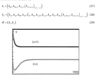
In Figure 1 we have plotted C t

( )

versus t for the chemo radiation model

and C t

( )

versus t for the quadrapeutics model. All rate constants equal to 1,

except k21=10,k65=10,k11,2=20. Also X =1. This supports the proof of

Theorem 1 that if you make the nanobubble kill rate k21 sufficiently big, then

quadrapeutics outperforms chemo radiation. I have iterated the Euler maps

(

,

) (

,

)

(

,

)

cr cr

H C D = C D +hf C D (25)

(

, , , ,

) (

, , , ,

)

(

, , , ,

)

q q

H C D G M N = C D G M N +hf C D G M N (26)

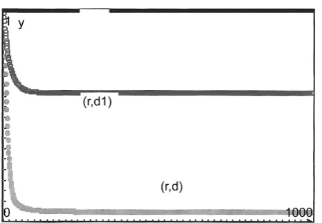
where h is the step size and equal to 0.02. There are 1000 iterations. The numer-ical analysis indicated, that C t D t G t M t

( ) ( ) ( ) ( ) ( )

, , , ,N t for the quadrapeutics

system converged, when t goes to infinity. And similarly for C(t),D(t) of the chemo radiation model, see Figure 1 and Figure 2.

Theorem 1. Assume, that aˆk98−k28−k X27 <0. There exist positive values of the rate constants kij, such that (24) holds and the singular points are all

pos-itive and stable.

Proof. Let K be defined by

{

}

(

)

1 82, 10,2, 11,2, 11 2 ,2i _i_1, _,_n

k = k k k k + ₌ _ (27)

{

}

(

)

2 21, 23, 98, 28, 27, 54, 2,10, 2,11, 65, 25, 26, 2,10 2i, 2,11 2i _i _1, _,_n

k = k k k k k k k k k k k k + k + ₌_ (28)

(

1, 2

)

[image:4.595.219.540.453.711.2]

K = k k (29)

Figure 1. (r, c1) is C(t) versus t for the chemo radiation

(5)

[image:5.595.259.492.65.226.2]

Figure 2. (r, d1) is D(t) versus t for the chemo radiation system and (r, d) is D(t) versus t for the quadrapeutics system.

Define

0 82 82

k =tk (30)

0 10,2 10,2

k =tk (31)

0 11,2 11,2

k =tk (32)

0

11 2 ,2i 11 2 ,2i 1, ,

k + =tk + i=  n t∈ (33)

when ∗ =n. Here

0 0 0 0

82, 10,2, 11,2, 11 2 ,2i

k k k k + ∈+ (34)

1, , .

i=  n Notice that

(

0,, 0

)

is a singular point of f, when t=0. The rate constants kij in k2 are positive real numbers. Also note that D f1 *0 is an

isomorphism. Here

1

cr

q

n    ∗ =    



(35)

For instance in f

{ }

1 0 ij _{i j}_, _1, _,_n D f = b ₌

 (36)

is an isomorphism, where b11=aˆ, b2,2= −k2,10, b3,3= −k2,11, b4,4 = −

(

k65+k25

)

,

5,5 26,

b = −k b5,4 =k65, b66= −k2,13,,bn+5,n+5 = −k2,11 2+ n, all other bij =0.

So there exist k

C maps, k≥5,

* *

*: *

p s

c V ⊂ → (37)

such that

( )

(

)

( )

(

)

* * * , * 0 * ˆ* 0, , 0

f c K K = c K =  (38)

(6)

Also

7 2

cr cr

p = s = (39)

14 5

q q

p = s = (40)

(

)

14 3 5

)

(

)

2 2, 2,10 2, 2,11 2 _1, _,

n j q

i i _i _n _j

1

ˆ n j_, n j _, n j _0.

n j

K − = k − k − k − = V* above is an open subset containing Kˆ* in *

p

 . Define

(

* *

(

*,0 *

)

* * 1 , 2

d t =c tk k (49)

For the chemo radiation model we let

* 0 * 0 * 0 *i 0

I

G M N

d = d = d = d = (50)

1, , .

i=  n For the quadrapeutics model we let _d_*Ii =0,_i=1,, ._n And for the multipeutics model we let

{

}

* 0 1, , 0, ,

i

I

d = i= − +n j  n j∈  n (51)

Differentiate (48) with respect to t to get

*

1 0

d f

D f

t t

∂ ∂

 _{ + =}

 _∂  _∂

  (52)

Thus

( )

0

*

82

1 0

ˆ

C

d

k

t a

∂

= −

∂ (53)

(7)

(

)

21 * * 23 * * 98 28 27 * 82 2,10 2 * * 1

0

i n

I

C N C D C C

i i

k d d k d d k k k X d k k ₊ d d

=

− − + − − + −

∑

= (54)

Differentiate this with respect to t to get

* * * *

21 * * 23 * *

C N C D

N C D C

d d d d

k d d k d d

t t t t

∂ ∂  ∂ ∂ 

− _ + _− _ + _

∂ ∂ ∂ ∂

    (55)

0

* * *

82 2,10 2 * *

1

ˆ 0

i i

I

C n C

I C i

i

d d d

a k k d d

t = + t t

 

∂ ∂ ∂

+ + − _ + _=

∂

∑

_ ∂ ∂ _ (56)

Also differentiate this equation with respect to t to find

2 2

* * * *

21 2 * 2 * 2

C C N N

N C

d d d d

k d d

t t t t ∂ ∂ ∂ ∂  − _ + + _ ∂ ∂ ∂ ∂

  (57)

2 2

* * * *

23 2 * 2 * 2

C C D D

D C

d d d d

k d d

t t t t ∂ ∂ ∂ ∂  − _ + + _ ∂ ∂ ∂ ∂

  (58)

2 2

* * * *

2,10 2 2 * * 2

1 2 i i i I I C C n I C i i

d d d d

k d d

t t t t + = ∂ ∂ ∂ ∂  −  _∂ + _∂ _∂ + _∂   

∑

(59)

2 * 2 ˆ 0 C d a t ∂ + =

∂ (60)

From this equation it follows that

( )

2

( )

2 2 2

1

2 0 2 0 2 0 2 0

C

C C C

q

cr d n

d d d

t t t t

∂

∂ ∂ ∂

= > > >

∂ ∂ ∂  ∂ (61)

anticipating that

( )

t k t k

+ +

∂ ₌ _> ∂ ₌ _>

∂ ∂ (64)

1, , .

i=  n The third equality holds for ∗ =q,1,, .n The fourth equality holds

t s

C d d

d t v v s

t t  ∂ ∂  = _ + _ ∂ ∂  

∫ ∫

(65)

So

( )

1

( )

C C C

q n

d t >d t >>d t (66)

(8)

( )

2

( )

2 1

( )

2

1 0 0 2 2

1

d d 0

2

C C

t s _q

C C

q

d d

d t d t v v v s ct

t t

∂ ∂ 

− = _ − _ ≥ >

∂ ∂

 

∫ ∫

(67)

because a positive function on a compact interval

[ ]

0,

δ

assumes a minimum 0

c> . The other inequalities follow in the same way. And this proves all the

in-equalities in (24) except * * q cr

C <C . Henceforth assume

2,10 2i 11 2 ,2i 2,11 2i 0

k ₊ =k ₊ =k ₊ = (68)

1, , .

i=  n Finally differentiate (57) to (60) with respect to t to get

2 2

* * * *

21 2 2

3

C N C N

d d d d

k t t t t ∂ ∂ ∂ ∂  − _ + _ ∂ ∂ ∂ ∂

  (69)

2 2

* * * *

23 2 2

3

C D C D

d d d d

k t t t t ∂ ∂ ∂ ∂  − _ + _ ∂ ∂ ∂ ∂

  (70)

3 * 3 ˆ 0 C d a t ∂ + =

∂ (71)

when t=0. But

( )

* ₀ * ₀ ₀

M N

d d

t t

∂ ∂

= =

∂ ∂ (72)

However when ∗ =q

( )

2 *

2 0 0

N

d

t

∂ _>

∂ (73)

To see this differentiate (17) twice with respect to t to find

(

)

2 *

( )

*

( )

*

( )

65 25 2 0 2 54 0 0 0

M D G

d d d

k k k

t t

t

∂ ∂ ∂

+ = >

∂ ∂

∂ (74)

If we now differentiate (18) twice with respect to t we find

( )

2 2

* *

26 2 0 65 2 0 0

N M

d d

k k

t t

∂ ₌ ∂ _>

∂ ∂ (75)

which is what we sought to show. Furthermore

(

65 25

) ( )

* 54 * *

( )

0

M D G

k +k d t =k d ⋅d t > (76)

and

( )

65

_{( )}

*

( )

*

21 * 26

0

M N

C k d t d t

k d t k

= >

+ (77)

when t>0 and small. Differentiate (15) twice with respect to t when ∗ =cr q, to get

2

* * * * *

2,10 2 2 23 2 54

D C D D G

d d d d d

k k k

t t t t

t

∂ ∂ ∂ ∂ ∂

− = +

∂ ∂ ∂ ∂

∂ (78)

Now 2 * * * 23 2 ˆ 2

C C D

d d d

a k t t t ∂ ∂ ∂ = ∂ ∂

(9)

Also

( )

₍

₎

3

65 54

* * * *

21 3

26 65 25

2

ˆ 0 3

C C D G

k k

d d d d

a k

t k k k t t

t

 

∂ ∂ ∂ ∂

= _ _

∂ + ∂ ∂

∂ _ _ (80)

* * *

23 23

1

3 2

ˆ

C D D

d d d

k k

a t t t

 ∂ ∂ ∂

+ _ _

∂ ∂ ∂

  (81)

* * * * *

23 23 54

2,10

1

3 2 2

C C D D G

d d d d d

k k k

k t t t t t

 

∂ ∂ ∂ ∂ ∂

− _ + _

∂ _ ∂ ∂ ∂ ∂ _ (82)

where we have evaluated in t=0 on the right hand side. So if

(

21 65

)

32

26 65 25 2,10

2 3 2

3 k k k 0

k k +k − k > (83)

we have

( )

3

( )

3

3 3

C C

q

cr d

d

t t

∂ ∂

>

∂ ∂ (84)

when t=0 and hence also for small t>0. The fundamental theorem of cal-culus applied three times gives

( )

3 *

( )

2 *

( )

*

( )

* 0 0 0 3 d 2 0 d 0 d

C C C

t s v

C d d d

d t u u v s

t

t t

  ∂ ∂  ∂ 

= _  _∂ + _∂  + _∂ _

 

∫ ∫ ∫

(85)

So

( )

C C

cr q

d t >d t (86)

for small t>0 and the theorem follows in the same way as (67). Define the matrices

* *

*c id *c

B=Df −

λ

A=Df (87)

and then write the definition of the determinant

( )

( ) ( ) 1, 1 ,

det 1

p

I

p p S

B σ B_σ B _σ

σ∈

=

∑

−  (88)

is odd. This formula shows immediately that

( )

1

(

11

)

0

det 1 , ,

p

p p i

i pp

i

B λ a A A λ

− =

= − +

∑

_ (89)

where ai is a polynomial in A11,,App, and hence is smooth in A11,,App.

You can prove this by induction. Now apply the continuous dependence of roots of a polynomial on its coefficients to show that d t*

( )

is stable for f*, when t

is small, see [19]. □

Remark. If the quadrapeutics chemo rate is

] [

10,2 10,2 0,1

q cr

k =k

α α

 ∈ (90)

and the x ray rate is

] [

27 27 0,1

q cr

(10)

where

,0 ,0

10,2 10,2 10,2 10,2

q q cr cr

k =tk k =tk (92)

while aˆ=k98−k28−k X27 <0. Here ,0 ,0 10,2, 10,2 q cr

k k ∈+ (93)

Then by taking k21 big we find

( )

3 3

3 0 3 0

C C

q cr

d d

t t

∂ ∂

<

∂ ∂ (94)

since

( )

3

ˆ 0

C q d a

t

∂

→ +∞

∂ (95)

as k21→ +∞. Hence

( )

C C

q cr

d t <d t (96)

for small t>0, when we impose (90) and (91), arguing as in the proof of theo-rem 1.

Experimentally this is what you see, that quadrapeutics can outperform che-mo radiation even if we take the cheche-mo radiation doses smaller, see [1][13][14] [15].

Consider also the system (1) to (13) with

2C+X →0 (97) replacing (7). The ODE s are the same (15) to (19) except (14), which is

(

)

2

21 23 98 28 82 27 2,10 2

1

2

n

i i

i

C k C N k C D k k C k k X C k ₊ C I

=

′ = − ⋅ − ⋅ + − + − ⋅ −

∑

⋅ (98)

We are now going to find candidates of the positive singular points of the dif-ferent systems. We start with f and assume that all kij are positive. (19) gives

11 2 ,2

2,10 2 2,11 2 i i

i i

k I

k C k

+

+ +

=

+ (99)

when C>0 and (18) gives

65

21 26 k M N

k C k

=

+ (100)

(16) and (17) give

(

)

11,2 2,11 65 25 0

k −k G− k +k M = (101)

or

(

)

(

11,2 65 25

)

2,11

1

G k k k M M

k α β

= − + = + (102)

Also

10,2

23 54 2,10 k

D

k C k G k

=

(11)

Insert these formulas in (14)

10,2 65

21 23

21 26 23 54 2,10

k k M

k C k C

k C k k C k G k

− −

+ + + (104)

(

)

(

)

(

k98 k28 k X27 1 δ 2C 1

)

C

+ − − + − ₍₁₀₅₎

11 2 ,2

2,10 2 82

=1 2,10 2 2,11 2

= 0

n

i i

i i i

k

k C k

+ +

− +

+

∑

(106)

0,1

δ = . Insert the formula for D in M′ =0 to get

(

)

10,2

54 65 26

23 54 2,10

0

k

k G k k M

k C+k G+k − + = (107)

We can isolate C in this equation to find

2

aM bM c

C

M

+ +

= ₍₁₀₈₎

where

(

)

54

65 25 2,11 23

k

a k k

k k

= + ₍₁₀₉₎

and

54 10,2 54 2,10 11,2 23 2,11 2,11 23 23

k k k k

b k

k k k k k

 

= − −_ + _

  (110)

Finally

(

)

54 10,2 11,2

23 2,11 65 25 k k k c

k k k k

=

+ (111)

We now get by multiplying with the product of the denominators in (104), (105) and (106)

(

) (

)

21 65 23 54 2,10 2,10 2 2,11 2 1

n

i i

i

k Ck M k C k G k k ₊ C k ₊

=

− + +

∏

+ (112)

(

)

(

)

23 10,2 21 26 2,10 2 2,11 2 1

n

i i

i

k Ck k C k k ₊ C k ₊

=

− +

∏

+ (113)

(

)

(

)

(

)

(

k82 k98 k28 k X27 1 δ 2C 1 C

)

(

k C21 k26

)

+ + − − + − + ₍₁₁₄₎

(

23 54 2,10

) (

2,10 2 2,11 2

)

1

n

i i

i

k C k G k k ₊ C k ₊

=

⋅ + +

∏

+ (115)

(

)

2,10 2 11 2 ,2 2,10 2 2,11 2

1 1,

n n

i i j j

i j j i

k + Ck + k + C k +

= = ≠

 

−  + 

 

∑

∏

(116)

(

k C23 k G54 k2,10

)

(

k C21 k26

)

0

⋅ + + + = (117)

If we now insert the formulas for G C, and multiply with Mn+3,

δ

=0 or

4

, 1,

n

)

2 n+4

(

δ

=1

)

in M, such that a positive singular point

(12)

will have p M

( )

=0. Let δ =1. Then we have

Theorem 2. For δ =1, there exist rate constants kij >0, such that (24)

holds and all equilibria are positive and stable.

Proof. Now let

98 28

ˆ

a=k −k (119)

and assume that it is negative. Then

( )

820 * ₀ ˆ C k d t a ∂ = −

∂ (120)

is the same for all treatments. But now the first coordinate of formula (48) be-comes

( )

2

21 * * 23 * * * 27 * 82 2,10 2 * * 1

ˆ 2 i 0

n

I

C N C D C C C

i i

k d d k d d ad k X d k k ₊ d d

=

− − + − + −

∑

= (121)

So

( )

2 2 2

* * * * *

21 * *

2 2

ˆ 0 2

C C C N N

N C

d d d d d

a k d d

t t t

t t

 

∂ ₌ ∂ ₊ ∂ ∂ ₊ ∂

 _∂ _∂ _∂ 

∂ _ ∂ _ (122)

2 2

* * * *

23 2 * 2 *

C C D D

D C

d d d d

k d d

t t t

t

∂ ∂ ∂ ∂ 

+ _ + + _

∂ ∂ ∂

∂

  (123)

2 2

* * * *

2,10 2 2 * *

1 2 i i i I I C C n I C i i

d d d d

k d d

t t t

t + = ∂ ∂ ∂ ∂  + _ + + _ ∂ ∂ ∂ ∂  

∑

(124)

2 * 27 4 C d k X t ∂  + _ _ ∂

  (125)

and when k2,10 2+ i=k2,11 2+ i=k11 2 ,2+ i =0,i=1,, .n

( )

3 2 2

* * * * *

21

3 2 2

ˆ 0 3

C C N C N

d d d d d

a k

t t

t t t

 

∂ ₌ ∂ ∂ ₊∂ ∂

 _∂ _∂ 

∂ _ ∂ ∂ _ (126)

2 2

* * * *

23 2 2

3

C D C D

d d d d

k t t t t ∂ ∂ ∂ ∂  + _ + _ ∂ ∂ ∂ ∂

  (127)

2 * * 27 2 12 C C d d k X t t ∂ ∂ + ∂

∂ (128)

We can now take k21 big and argue as in theorem 1. □

3. The Chemo Radiation Model

Consider the mass action kinetic system 0

C+ →D (129)

(

1+

δ

)

C+ →X 0,

δ

=0,1 (130) 2

C C (131)

0

C (132)

0

(13)

Here the complexes are C

( )

(

)

23 10,2 2,10

1 2 1

, k k C D k k k X C C

f C D

k C D k k D

δ

 ₋ _{⋅ +} ₋ ₋ ₊ ₋ 

 

=

 ₋ _{⋅ +} ₋ 

  (134)

all kij >0.

This system with δ =0 is similar to the reduced system from [17].

GF→C (135)

0

C+GI → (136)

2

C→ C (137)

0

GF (138)

0

GI (139)

0

C (140)

where we have added the last reaction. The complexes are C

( )

1 =GF,

( )

2 ,

C =C C

( )

3 = +C GI, C

( )

4 =0, C

( )

5 =2 ,C C

( )

6 =GI. The vector field is

(

k GF k C GI k k C k

g C GF GI k k k GF

k C GI k k GI

 − ⋅ + − + 

 

=_ − + _

 ₋ _⋅ ₊ ₋ 

 

(141)

We can assume that GF is at equilibrium

14

21 41 k GF

k k

=

+ (142)

The reduced system is then

(

)

43

(

52 42

)

43 64 46

ˆ , k k C GI k k C

g C GI

k C GI k k GI

 − ⋅ + − 

=  ₋ _⋅ ₊ ₋ 

  (143)

21 14 24 21 41 k k

k k

= +

+ (144)

We shall find the singular points of the chemo radiation system. D′ =0 gives

10,2

23 2,10 k D

k C k

=

+ (145)

when C>0 and then C′ =0 amounts to

(

)

(

)

(

)

10,2

82 23 98 28 27

23 2,10

1 2 1 0

k

k k C k k k X C C

k C k

δ

− + − − + − =

+ (146)

which is equivalent to

23 98 28 27 23

*

23 2,10 23

c

k D k k k X k C

A Df

k D k k C

− + − − − 

= = _ ₋ ₋ ₋ _

  (151)

when δ =0 and when δ =1 it is

(

)

23 98 28 27 23

*

23 2,10 23

4

c

k D k k k XC k C

A Df

k D k k C

− + − − − 

= = _ ₋ ₋ ₋ _

 

 ₍₁₅₂₎

If δ =0

98 28 27

ˆ 0

a=k −k −k X < (153)

and

(

C D,

)

is a positive singular point, then

(

)

23 2,10 23

ˆ ˆ

traceA 0 detA ak C k k D a 0

σ

= < = − + − > ₍₁₅₄₎

hence this is a stable, positive singular point. Consider the chemo radiation system where

10,2 23 98 13 1 1

k = k = X =

δ

= (155)

and all other kij =1. Then the cubic polynomial giving candidates of singular points is

3 2

2C 10C 10C 1 0

− + − + = ₍₁₅₆₎

and this gives three singular points

(

)

(

)

(

)

0.112, 20.68

, 1.21,10.41

3.677, 4.918

C D

  =   

(157)

where we have used that

10,2

23 2,10 k D

k C k

=

+ (158)

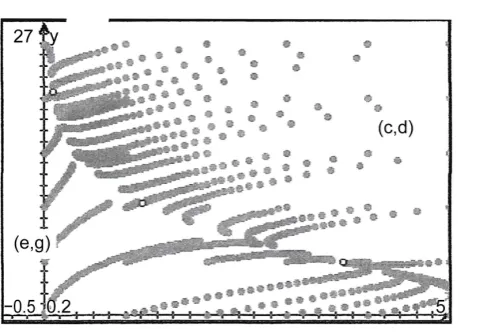
It is a simple matter to check that the first and last of these are stable equilibria and the middle is an unstable saddle by computing the trace and determinant of the linearization of fq in the singular points. I have plotted a phase portrait for

these values of the parameters in Figure 3.

4. The Quadrapeutics Equilibrium Equation

We shall find the quadrapeutics equilibrium equation too.

Theorem 3. Suppose δ =0. There exists a polynomial of degree atmost six

( )

6

0

i

i i

i

s M q M q

=

∑

∈ (159)

such that if

(

C D G M N, , , ,

)

is a positive singular point of f_q then

( )

0

(15)

[image:15.595.260.501.62.229.2]

Figure 3. A tristable chemo radiation system. There are three singular points marked with a circle.

Proof. Isolate D, G, M, N from (15), (16), (17), (18) and insert it in

(

)

1 , , , , 0

q

f C D G M N = to find

(

, ,

)

21 65

(

23 54 2,10

)

p C G M = −k Ck M k C+k G+k (161)

(

)

23 10,2 21 26 k Ck k C k

− + ₍₁₆₂₎

(

)

(

)

(

)

(

k82 k98 k28 k X27 1 δ 2C 1 C

)

+ + − − + − ₍₁₆₃₎

(

k C21 k26

)

(

k C23 k G54 k2,10

)

0

⋅ + + + = ₍₁₆₄₎

where we have multiplied with

(

k C21 +k26

)

(

k C23 +k G54 +k2,10

)

(165)

We shall now insert

2

aM bM c

C G M

M

α

β

+ +

= = + (166)

where

65 25

2,11

k k

k

α= − + (167)

11,2

2,11 k k

β

= ₍₁₆₈₎

in the polynomial p. Compute

6 3 3

0

i i i

M C a M

=

∑

 (169)

where

3 6

a =a (170)

2 5 3

a = a b (171)

(

2 2

)

4 3

a = ab +a c (172)

3 3 6

(16)

(

2 2

)

2 3

a = ac +b c (174)

2 1 3

a = bc (175)

3 0

a =c (176)

Now define

(

)

3

(

)

1 , , 21 65 23 54 2,10

p C G M =M −k Ck M k C+k G+k (177)

and this is

( )

2

1 1 , ,

aM bM c

s M p M M

M

α

β

 + + 

= _ + _

  (178)

Also put

(

)

3

(

)

2 , , 23 10,2 21 26

p C G M =M −k Ck k C+k (179)

and this is

( )

2

2 2 , ,

aM bM c

s M p M M

M

α

β

 + + 

= _ + _

  (180)

Finally set

(

)

3

(

)(

)

(

)

3 , , 82 ˆ 21 26 23 54 2,10

p C G M =M k +aC k C+k k C+k G+k (181)

which is

( )

2

3 3 , ,

aM bM c

s M p M M

M

α

β

 + + 

= _ + _

  (182)

So

)

21 65 54 ) 2,10

k aM bM c k M k

α

M

β

k

− + + + + ₍₁₈₅₎

(

2 6 2 4 2 2 5 4 3

)

21 65 23 2 2 2

k k k a M b M c M abM acM bcM

= − + + + + + ₍₁₈₆₎

(

)

(

)

(

)

2 3

21 65 54

2 3

21 65 54 2,10

k k aM bM c M k M

k k aM bM c M k k

α β

− + +

− + + + (187)

Write

( )

6

1

0

i i i

s M a M

=

∑

₍₁₈₈₎

Then by the previous computation

(

)

6 21 65 23 54

a = −k ak k a k+

α

(189)

(

)

(

)

5 21 65 23 54 21 65 54 23 2,10

a = −k bk k a+k

α

−k ak k

β

+k b k+ (190)

(

)

(

)

4 21 65 23 54 21 65 54 23 2,10 21 65 23

(17)

(

)

3 21 65 54 23 2,10 21 65 23

a = −k ck k β+k b+k −k k k bc (192)

2 2 21 65 23

a = −k c k k (193)

1 0

a = (194)

0 0

a = (195)

Now compute

( )

3

(

)

2 23 10,2 21 26

s M =M −k Ck k C+k (196)

2 4 2 2 2 3 2

3

23 10,2 21 2

2

26

2 2 2

a M b M c abM acM bcM

M k k k

M

aM bM c

k

M

 + + + + +

= − _

 

+ +

+ _



(197)

(

2 5 2 3 2 4 3 2

)

23 10,2 21 2 2 2

k k k a M b M c M abM acM bcM

= − + + + + + ₍₁₉₈₎

(

4 3 2

)

23 10,2 26

k k k aM bM cM

− + + ₍₁₉₉₎

Write

( )

6

2

0 i i i

s M b M

=

∑

₍₂₀₀₎

and by the computation above

6 0

b = (201)

2 23 10,2 21 26 23 10,2 21

b = −k ck k b+k −k bk k c (205)

2 1 23 10,2 21

b = −k c k k (206)

0 0

b = (207)

Now consider

(

)

3 2

3 , , 21 23ˆ 21 54ˆ

p C G M =k k aC +k k aC G (208)

2 2

21ˆ 2,10 26 23ˆ k aC k k k aC

+ + ₍₂₀₉₎

26 54 ˆ 26 2,10ˆ k k GaC k k aC

+ + ₍₂₁₀₎

2

82 21 23 82 21 54 k k k C k k k CG

+ + ₍₂₁₁₎

82 21 2,10 82 26 23 k k k C k k k C

+ + (212)

82 26 54 82 26 2,10 k k k G k k k

+ + (213)

Name these 12 summands d1,,d12. Now 6 3

1 21 23 0

ˆ i

i i

M d k k a a M

=

∑

 (214)

(18)

(

)

(

3 2 6 2 4 2 2 5 4 3

2 21 54ˆ 2 2 2

M d =k k a α a M +b M +c M + abM + acM + bcM (215)

(

2 5 2 3 2 4 3 2

)

2 2 2

(

)

3 5 4 3 4 3 2

8 82 21 54

M d =k k k α aM +bM +cM +β aM +bM +cM (222)

Combine

(

)

(

)

(

)

3 4 3 2

9 10 82 21 2,10 82 26 23

M d +d = k k k +k k k aM +bM +cM (223)

The last two ds give

(

)

3 4 3

11 82 26 54

M d =k k k αM +βM (224)

3 3

12 82 26 2,10

M d =k k k M (225)

Write

( )

6

3

0 i i i

s M c M

=

∑

(226)

Then we find from the above computations

(

)

2

6 ˆ 21 23 54

c =aa k k a+k α (227)

and

(

)

2 2 2

5 21 23ˆ3 21 54ˆ 2 21ˆ 2,10

c =k k a a b+k k a α ab+βa +k ak a (228)

2 2

26 23ˆ 82 21 23 82 21 54 26 54ˆ k k aa k k k a k k k a

α

k k a a

α

+ + + + ₍₂₂₉₎

Now collect terms

(

2 2

)

(

2

)

4 21 23ˆ3 21 54ˆ 2

c =k k a ab +a c +k k aα b + ac (230)

21 54ˆ 2 21ˆ 2,102 26 23ˆ2 k k a

β

ab k ak ab k k a ab

+ + + (231)

(

)

26 54ˆ 26 2,10ˆ k k a

α

b

β

a k k aa

+ + + (232)

(

)

82 21 232 82 21 54

k k k ab k k k

α

b

β

a

+ + + (233)

(

k k k82 21 2,10 k k k82 26 23

)

a k k k82 26 54α

(19)

We can also find

(

3

)

(

2

)

3 21 23ˆ 6 21 54ˆ 2 2

c =k k a abc b+ +k k a bcα β+ b + ac (235)

(

2

)

(

2

)

21ˆ 2,10 2 26 23ˆ 2

k ak b ac k k a b ac

+ + + + ₍₂₃₆₎

(

)

26 54ˆ 26 2,10ˆ k k a c

α β

b k k ab

+ + + ₍₂₃₇₎

(

2

)

(

)

82 21 23 2 82 21 54

k k k b ac k k k αc βb

+ + + + ₍₂₃₈₎

(

k k k82 21 2,10 k k k82 26 23

)

b k k k82 26 54β k k k82 26 2,10

+ + + + (239)

Now

(

2 2

)

(

2

)

2 21 23ˆ3 21 54ˆ 2

c =k k a ac +b c +k k a αc +β bc (240)

(

k ak21ˆ 2,10 k k a26 23ˆ

)

2bc k k a c26 54ˆβ

+ + + ₍₂₄₁₎

26 2,10ˆ 82 21 232 k k ac k k k bc

+ + ₍₂₄₂₎

(

)

82 21 54 82 21 2,10 82 26 23

k k k βc k k k k k k c

+ + + (243)

Also

2 2 2

1 21 23ˆ3 21 54ˆ 21ˆ 2,10

c =k k a bc +k k ac β+k ak c (244)

2 2

82 21 23 23 ˆ 26 k k k c k c ak

+ + (245)

Finally

3 0 21 23ˆ

c =k k ac (246)

The quadrapeutics polynomial is

( )

6

(

)

0

i i i i i

s M a b c M

=

∑

+ + (247)

□

If all rate constants kij =1,X =1 then

( )

5 4 3 23 2 3 1

2 8 10 0

4 2 8

s M = M − M + M − M + M− = (248)

This polynomium has three real roots 1

0.148638, , 2.32234

2

M = M = M = (249)

and two imaginary roots

0.514511 0.312089± i (250)

There are thus two candidates of singular points ( 1

2

M = does not give a

singular point).

(

, , , ,

) (

₍

0.661153, 0.423634, 0.702724, 0.148638, 0.089479

₎

)

1.85998, 1.27437, 3.64468, 2.32234, 0.812013

C D G M N = 

− −

 (251)

(20)

G=αM +β (252)

2

aM bM c

C

M

+ +

= ₍₂₅₃₎

10,2

23 54 2,10 k

D

k C k G k

=

+ + (254)

65

21 26 k M N

k C k

=

+ (255)

5. The Extended Quadrapeutics Model

This is the system (1) to (11) and the reactions 0

D C+ → (256)

N+D→D (257)

0

D → (258)

D→D (259)

taking into account, that plasmonic nanobubbles destroy the liposomes D and

thus the chemo therapeutic drug D is injected into the cytoplasm. But some of

the liposomes decay, producing chemo therapeutic drug. The complexes here are

( )

12 ,

( )

13 ,

( )

14 .

C = +N D C =D C = +D C The ODEs are

(

)

21 23 98 28 27 82 2,14

C′ = −k C N⋅ −k C D⋅ + k −k −k X C+k −k D C⋅ (260)

2,14 13,12 2,13 13,10

D′ = −k D C⋅ +k N D⋅ −k D+k D (261)

23 54 10,2 2,10 13,12 13,10

D′ = −k C D k D G⋅ − ⋅ +k −k D k− N D k⋅ − D (262)

54 11,2 2,11

G′ = −k D G⋅ +k −k G (263)

(

)

54 65 25

M′ =k D G⋅ − k +k M (264)

21 65 26 13,12

N′ = −k C N⋅ +k M−k N−k N D⋅ (265)

The vector field is denoted gq. Denote by gcr the vector field in (260), (261)

and (262) with the rate constants in (263), (264) and (265) all equal to zero and the rest positive.

Theorem 4. There exist positive values of the rate constants such that

* *

q cr

)

1 82, 10,2

cr

k = k k (269)

(

)

2 23, 98, 28, 27, 2,14, 2,13, 2,10, 13,10 cr

(21)

Define

(

1 , 2

)

(

1, 2

)

cr cr q q

cr q

K = k k K = k k (271)

and

(

* *

)

*

* 1 2 1

ˆ _, ₀

K = k k k = (272)

Use the implicit function theorem to find a mapping

18 6

:

q q

c V ⊂ → (273)

and

10 3

:

cr cr

c V ⊂ → (274)

such that

( )

(

)

( )

* * * , * 0 * ˆ* 0

g c K K = c K = (275)

and define

( )

(

*,0 *

)

* * 1 , 2

cr

d t c tk k

q 

= _{∗ = }

 (276)

,

q cr

V V are open subsets of  18, 10 respectively. For ∗ =cr let d_*G =d_*M

* 0. N d

= = _{By the implicit function theorem}

( )

* 0 0

D

d = (277)

Differentiate (262) and (261) with respect to t to get

0 10,2 *

2,10 13,10

D _k

d

t k k

∂ =

∂ + (278)

and

(

)

0 10,2 13,10 *

2,13 2,10 13,10

D _k _k

d

t k k k

∂ =

∂ +



(279)

Now differentiate (261) twice with respect to t to find

2 2

* * * *

2,13 2 13,10 2 2 2,14

D D D C

d d d d

k k k

t t

∂ ∂ ∂ ∂

= −

∂ ∂

 

(280)

and differentiate (262) with respect to t to get

2

* * * * *

23 54

2

2,10 13,10

2

D C D D G

d d d d d

k k

k k t t t t

t

 

∂ ∂ ∂ ∂ ∂

= − _ + _

+ ∂ ∂ ∂ ∂

∂ _ _ (281)

We also have

0 0

11,2 82

* *

2,11

ˆ

C G _k

k

d d

t a t k

∂ ∂

= − =

∂ ∂ (282)

the last equality when ∗ =q. We now get 2

* * * * * * *

23 2,14 21

2

1

2 2

ˆ

C C D D C C N

d d d d d d d

k k k

a t t t t t t

t

 

∂ ₌ ∂ ∂ ₊ ∂ ∂ ₊ ∂ ∂

 

 _∂ _∂ _∂ _∂ _∂ _∂ 

∂ _ _



(22)

so

( )

2

( )

2

2 0 2 0

C C q cr d d t t ∂ ∂ =

∂ ∂ (284)

and

(

)

2 65 54 * * * 2

26 65 25

2

N _k _k D G

d d d

k k k t t

t

∂ ∂ ∂

=

+ ∂ ∂

∂ (285)

where we have used that

( )

* ₀ ₀

M

d t ∂

=

∂ (286)

hence

( )

* ₀ ₀

N

d t ∂

=

∂ (287)

Finally

3 2 2

* * * * *

23

3 2 2

ˆ 3

C C D C D

d d d d d

a k

t t

t t t

 

∂ ₌ ∂ ∂ ₊∂ ∂

 _∂ _∂ 

∂ _ ∂ ∂ _ (288)

2 2

* * * *

2,14 2 2

3

D C D C

d d d d

k t t t t ∂ ∂ ∂ ∂  + _ + _ ∂ ∂ ∂ ∂     (289) 2 * * 21 2 3 C N d d k t t ∂ ∂ +

∂ ∂ (290)

and taking k21 big, this implies the theorem, arguing as in the proof of

theo-rem 1. □

From D′ =0 isolate

(

)

(

54 10,2 2,10 13,10 13,12

)

23

1

C k D G k k k D k N D

k D

= − ⋅ + − + − ⋅ ₍₂₉₁₎

and insert this in N′ =0 to get using

0 0

G=αM+β α< β > (292)

and

(

2,11

)

54 k M D k M

α

β

− =

+ (293)

(this equation follows from (263)), that

(

)

(

)

13,12 21 2 21 21 10,2 54 54

23 23 23 2,11

k k k k k k M

N N k M

k k k k M

α β

α

 +

+ _ + +

 (294)

(

)

2,10 13,10 2,11

21 26 13,12 65

23 54

0

k k k M

k k k k M

k k M

α

α β

 +

+ − + _+ =

+ _ (295)

0, .

M M

β

α

> ≠ − Let a be the coefficient to 2

N and let b M

( )

be the