Parallelization of formal concept analysis algorithms

Parallelization of formal concept analysis algorithms

Available from Sheffield Hallam University Research Archive (SHURA) at: http://shura.shu.ac.uk/24465/

This document is the author deposited version. You are advised to consult the publisher's version if you wish to cite from it.

Published version

KODAGODA, Gamhewage Nuwan (2018). Parallelization of formal concept analysis algorithms. Doctoral, Sheffield Hallam University.

Copyright and re-use policy

See http://shura.shu.ac.uk/information.html

P

ARALLELIZATION OF

F

ORMAL

C

ONCEPT

ANALYSIS ALGORITHMS

Gamhewage Nuwan Kodagoda

A thesis submitted in partial fulfilment of the requirements of Sheffield Hallam

University for the degree of Doctor of Philosophy

i

Abstract

Formal Concept Analysis provides the mathematical notations for representing concepts and concept hierarchies making use of order and lattice theory. This has now been used in numerous applications which include software engineering, linguistics, sociology, information sciences, information technology, genetics, biology and in engineering. The algorithms derived from Kustenskov's CbO were found to provide the most efficient means of computing formal concepts in several research papers. In this thesis key enhancements to the original CbO algorithms are discussed in detail. The effects of these key features are presented in both isolation and combination. Eight different variations of the CbO algorithms highlighting the key features were compared in a level playing field by presenting them using the same notation and implementing them from the notation in the same way. The three main enhancements considered are the partial closure with incremental closure of intents, inherited canonicity test failures and using a combined depth first and breadth first search. The algorithms were implemented in an un-optimized way to focus on the comparison on the algorithms themselves and not on any efficiencies provided by optimizing code.

One of the findings were that there is a significant performance improvement when partial closure with incremental closure of intents is used in isolation. However there is no significant performance improvement when the combined depth and breadth first search or the inherited canonicity test failure feature is used in isolation. The inherited canonicity test failure needs to be combined with the combined depth and breadth first feature to obtain a performance increase. Combining all the three enhancements brought the best performance.

ii

Acknowledgements

I am grateful to my research supervisor Prof. Simon Andrews of the Department of Computing, Faculty of Arts, Computing, Engineering and Sciences, Sheffield Hallam University for his guidance, untiring support and encouragement during this research.

I also wish to thank the management of SLIIT for sponsoring my PhD and providing me support to pursue my research work. I would like to specifically thank Prof Lalith Gamage, President/CEO of SLIIT and former Chairman of SLIIT Prof Sam Karunarathne for the support and encouragement they have extended to me during this period. I also wish to express my gratitude to the Deans of the Faculty of Computing, during this period, Prof Koliya Pulasinghe who is also my internal supervisor at SLIIT and Dr Malitha Wijesundara for their kind encouragement and support.

I wish to thank my parents for supporting me and guiding me to pursue an academic life, I am much indebted to them. My sister Neesha, for her continuous support and encouragement. She also put up with me and provided lodging during my annual visits to UK.

iii

Dedication

iv

Publications

The following research articles were published based on the research work carried out.

Kodagoda, Nuwan, and Pulasinghe, Koliya (2016). "Comparision Between Features of CbO based Algorithms for Generating Formal Concepts." International Journal of Conceptual Structures and Smart Applications (IJCSSA) 4.1 (2016): 1-34.

v

TABLE

OF

CONTENTS

1. INTRODUCTION ... 1

1.1INTRODUCTION ... 1

1.2RESEARCHQUESTIONS ... 3

1.3OBJECTIVESANDSTRUCTUREOFTHETHESIS ... 3

1.3.1METHODOLOGY ... 4

1.3.2FORMAL CONCEPT ANALYSIS ... 4

1.3.3COMPARISON OF EXISTING SERIAL ALGORITHMS ... 4

1.3.4SHARED MEMORY PARALLEL ALGORITHMS ... 5

1.3.5DISTRIBUTED MEMORY PARALLEL ALGORITHMS ... 5

1.4NEWFCAALGORITHMSPRESENTEDINTHISTHESIS ... 5

2. METHODOLOGY ... 7

2.1INTRODUCTION ... 7

2.2METHODOFSAMPLING ... 8

2.3STATISTICALSIGNIFICANCEOFEMPIRICALRESULTS ... 11

2.3.1INTRODUCTION ... 11

2.3.2ONE-WAY ANALYSIS OF VARIANCE ... 11

2.3.3 T-TEST FOR TWO SAMPLE ASSUMING UNEQUAL VARIANCES ... 14

2.4DETAILACTIVITIESUNDERTAKENINTHISRESEARCH ... 16

2.5BENCHMARKINGOFTHEIMPLEMENTATIONS ... 17

2.6UNITTESTINGTHEIMPLEMENTATIONS ... 18

2.7COMPARISONOFSERIALIMPLEMENTATIONSOFFCA ... 18

2.8EXPERIMENTALTESTINGOFPARALLELALGORITHMS ... 20

3. FORMALCONCEPTANALYSIS ... 22

3.1FORMALCONCEPTANALYSISBACKGROUND ... 22

3.2FCAALGORITHMS ... 27

3.3LIMITATIONSOFSERIALFCAALGORITHMS ... 28

3.4EXISTINGPARALLELFCAALGORITHMS ... 29

4. COMPARISIONOFFCASERIALALGORITHMS ... 30

4.1EXISTINGFCAALGORITHMS ... 30

4.2DETAILSOFTHEEIGHTCBOBASEDALGORITHMS ... 33

4.2.1CBO-FC-DF(CBO–FULL CLOSURE,DEPTH FIRST SEARCH ALGORITHM) ... 33

4.2.2CBO-PC-DF(CBO–PARTIAL CLOSURE,DEPTH FIRST SEARCH ALGORITHM) ... 36

4.2.3CBO-FC-DBF(CBO–FULL CLOSURE,COMBINED DEPTH FIRST AND BREADTH FIRST SEARCH ALGORITHM) ... 38

4.2.4CBO-FC-ICF-DF(CBO–FULL CLOSURE,INHERITED CANONICITY TEST FAILURE, DEPTH FIRST SEARCH ALGORITHM) ... 40

4.2.5CBO-PC-DBF(CBO–PARTIAL CLOSURE,COMBINED DEPTH FIRST AND BREADTH FIRST SEARCH ALGORITHM) ... 42

4.2.6CBO-PC-ICF-DF(CBO–PARTIAL CLOSURE,INHERITED CANONICITY TEST FAILURE, DEPTH FIRST SEARCH ALGORITHM) ... 43

4.2.7CBO-FC-ICF-DBF(CBO–FULL CLOSURE,INHERITED CANONICITY TEST FAILURE, COMBINED DEPTH FIRST AND BREADTH FIRST SEARCH ALGORITHM) ... 44

4.2.8CBO-PC-ICF-BF(CBO–PARTIAL CLOSURE,INHERITED CANONICITY TEST FAILURE, COMBINED DEPTH FIRST AND BREADTH FIRST SEARCH ALGORITHM) ... 45

4.3IMPLEMENTATIONDETAILS ... 45

vi

4.4.1INTRODUCTION ... 48

4.4.2STATISTICAL SIGNIFICANCE OF THE EMPIRICAL RESULTS ... 50

4.4.3IMPACT OF THE THREE ENHANCEMENTS IN ISOLATION ... 52

4.4.3.1INTRODUCTION ... 52

4.4.3.2THE IMPACT OF USING PARTIAL CLOSURES WITH INCREMENTAL CLOSURE OF INTENTS ... 53

4.4.3.3THE IMPACT OF USING COMBINED DEPTH FIRST AND BREADTH FIRST SEARCH ... 54

4.4.3.4THE IMPACT OF THE INHERITED CANNOCITY TEST FAILURE ... 55

4.4.3.5THE IMPACT OF THE COMBINATION OF THE PARTIAL CLOSURE WITH THE INCREMENTAL CLOSURE OF INTENTS JOINED WITH THE COMBINED DEPTH FIRST AND BREADTH FIRST SEARCH ... 57

4.4.3.6THE IMPACT OF THE COMBINATION OF THE COMBINED PARTIAL CLOSURE WITH THE INCREMENTAL CLOSURE OF INTENTS JOINED WITH THE INHERITED CANNOCITY TEST FAILURE ... 58

4.4.3.7THE IMPACT OF THE COMBINATION OF THE COMBINED DEPTH FIRST AND BREADTH FIRST SEARCH JOINED WITH THE INHERITED CANNOCITY TEST FAILURE ... 58

4.4.3.8THE EFFECT OF THE COMBINATION OF ALL THREE FEATURES ... 59

4.4.4ANALYSIS OF THE EFFECTS OF THE THREE VARIATIONS ... 60

4.4.5VALIDATING THE RESULTS OF INSTRUMENTING CLOSURES AND INTERSECTIONS ... 62

4.5 ANALYSISOFTHEEIGHTCBOBASEDALGORITHMS ... 65

4.5.1INTRODUCTION ... 65

4.5.2ANALYSIS OF CBO-FC-DF(CBO) ... 66

4.5.3ANALYSIS OF CBO-PC-DF(IN-CLOSE) ... 67

4.5.4ANALYSIS OF CBO-PC-DBF(IN-CLOSE2) ... 67

4.5.5ANALYSIS OF CBO-FC-ICF-DBF(FCBO) ... 68

4.5.6ANALYSIS OF CBO-FC-DBF ... 69

4.5.7ANALYSIS OF CBO-FC-ICF-DF ... 69

4.5.8ANALYSIS OF CBO-PC-ICF-DF ... 69

4.5.9ANALYSIS OF CBO-PC-ICF-DBF(IN-CLOSE3) ... 70

5. SHAREDMEMORYPARALLELALGORITHMS ... 72

5.1. DIFFERENTTYPESOFPARALLELMACHINES ... 72

5.2. DEVELOPINGPARALLELPROGRAMS ... 73

5.3 SELECTIONOFTECHNOLOGYSTACKFORSHAREDMEMORY PARALLELIMPLEMENTATION ... 74

5.4. INTRODUCTIONONTHESHAREDMEMORYALGORITHMS ... 75

5.5. NAIVEPARALLELALGORITHMFORIN-CLOSE3 ... 75

5.5.1INTRODUCTION ... 75

5.5.2PERFORMANCE EVALUATION OF NAÏVE PARALLEL IN-CLOSE3 ... 76

5.6. EXISTINGPARALLELFCAALGORITHMS ... 78

5.7. TWOADDITIONALPARALLELVARIATIONSOFIN-CLOSE3 ... 81

5.8 COMPARISONOFTHEFOURPROPOSEDPARALLELVARIATIONS OFIN-CLOSE3 ... 85

5.9 COMPARISONWITHPFCBO ... 91

5.9.1INTRODUCTION ... 91

5.9.2STATISTICAL SIGNIFICANCE OF THE EMPIRICAL RESULTS ... 92

5.10.IMPLEMENTATIONDETAILS ... 94

5.11.IMPLEMENTATIONDETAILSOFTHENAÏVEPARALLEL IN-CLOSE3ALGORITHM ... 96

vii

5.13.IMPLEMENTATIONDETAILSOFTHEQUEUEPARALLEL

IN-CLOSE3ALGORITHM ... 98

5.14.OPTIMISINGCARRIEDOUTINTHEPARALLEL IMPLEMENTATIONS ... 99

6. DISTRIBUTEDMEMORYPARALLELALGORITHMS ... 103

6.1. DISTRIBUTEDMEMORYMACHINES ... 103

6.2 DISTRIBUEDMEMORYPARALLELPROGRAMS ... 105

6.3 EXISTINGPARALLELFCAALGORITHMS ... 105

6.4. PROPOSEDDISTRIBUTEDMEMORYALGORITHMS ... 106

6.5. DISCUSSIONOFTHEDISTRIBUTEDMEMORYIMPLEMENTATION OFIN-CLOSE3 ... 113

6.5.1. EXPERIMENTS CARRIED OUT ... 113

6.5.2. VALIDATION AND TESTING OF THE IMPLEMENTATION ... 115

6.5.3. OPTIMIZATION OF THE IMPLEMENTATION ... 115

7. CONCLUSIONANDFUTUREWORK ... 116

7.1. CONCLUSION ... 116

7.1.1.MAJOR CONTRIBUTIONS OF THE THESIS ... 116

7.1.2.ANALYSIS OF SERIAL CBO BASED ALGORITHMS ... 116

7.1.3.PARALLELIZATION OF IN-CLOSE3 ... 117

7.1.4.ANALYTICAL ANALYSIS OF SERIAL CBO BASED ALGORITHMS ... 118

7.2. DISCUSSION ... 118

7.2.1.DEBUGGING PARALLEL PROGRAMS ... 118

7.2.2.CROSS PLATFORM DEVELOPMENT AND PARALLEL ARCHITECTURES USED FOR EXPERIMENTS ... 119

7.3. FUTUREWORK ... 119

APPENDIX –A–SERIAL ALGORITHM IMPLEMENTATIONS ... 127

APPENDIX –B–DISTRIBUTED MEMORY ALGORITHM IMPLEMENTATIONS ... 130

viii

LIST

OF

TABLES

TABLE2.1,STATISTICALANALYSISCARRIEDOUTFORONERAW

EXPERIMENTALRESULT ... 10 TABLE2.2,EMPIRICALTIMING(SECONDS)FOREACHSERIALALGORITHMRUNNING

THEMUSHROOMDATASET ... 12 TABLE2.3,ONEWAYANALYSISOFVARIANCE(ONEWAYANOVA)FORDATASETIN

TABLE2.2 ... 12 TABLE2.4,T-TEST:TWO-SAMPLEASSUMINGUNEQUALVARIANCESFORTHETWO

FASTESTALGORITHMS (RANK1ANDRANK2INTABLE2.2)IN-CLOSE3

ANDFCBO ... 15 TABLE2.5,SAMPLETESTCASESFORACTUALDATASETS

(TIMINGINSECONDS) ... 17 TABLE2.6,RANDOMBENCHMARKINGDATASETS ... 18 TABLE4.1,EIGHTVARIATIONSOFCBO ... 32 TABLE4.2,LISTOFFUNCTIONSUSEDTOIMPLEMENTTHE

COMMONCODEBLOCKS ... 34 TABLE4.3,MAINDATASTRUCTURESUSEDINTHE

IMPLEMENTATIONS ... 46 TABLE4.4,TESTRESULTSFORREALWORLDDATASETS

(TIMEINSECONDS)WITH95%CONFIDENCELEVELS ... 47 TABLE4.5,RESULTSFORARTIFICIALDATASETSWHEREDENSITY

ISAVARIABLE, ... 49 TABLE4.6,RESULTSFORARTIFICIALDATASETSWHERE|G|IS

AVARIABLE,|M|=100(TIMINGINSECONDS)AND

DENSITY=5% ... 49 TABLE4.7,RESULTSFORARTIFICIALDATASETSWHERE|M|ISAVARIABLE,|G|=100

(TIMINGINSECONDS)ANDDENSITY=5% ... 50 TABLE4.8,ONE-WAYANALYSISOFTHEMAJORDATASETSUSEDINTHEANALYSIS ... 51 TABLE4.9,T-TESTFORTWOSAMPLEASSUMINGUNEQUALVARIANCESANALYSIS

OFTHEMAJORDATASETSUSEDINTHEANALYSIS ... 51 TABLE4.10,SPEEDUPOFTHECOMPARISONOFALGORITHMSFORTHEDENSITY–

N100M100D50S1000.CXT,OBJECTS-N100M100000D5S1000.CXT,

ATTRIBUTES–N2000M100D5S1000.CXT ... 61 TABLE4.11,COMPARISONOFCLOSURESANDINTERSECTIONSFORTHEREALDATASETS. .. 63 TABLE4.12,COMPARISONOFCLOSURESANDINTERSECTIONSFORARTIFICIALDATASETS. 64 TABLE4.13,ALGORITHMICCOMPLEXITYOFCODEBLOCKS ... 66 TABLE4.14,ANALYTICALRESULTSOBTAINED ... 70 TABLE5.1,AVERAGETIMEOBTAINEDFORDIFFERENTREALDATASETS,WITH95%

CONFIDENCELEVELS ... 77 TABLE5.2,AVERAGETIMEOBTAINEDFORDIFFERENTLARGEARTIFICIALDATASETS,

WITH95%CONFIDENCELEVELS ... 77 TABLE5.3,REALWORLDDATASETRESULTS (AVERAGETIMINGINSECONDS)FOR

ix

CORES=12WITH95%CONFIDENCELEVEL ... 85 TABLE5.4,ARTIFICIALDATASETRESULTS(AVERAGETIMINGINSECONDS)FOR

IN-CLOSE3ANDFCBOPARALLELALGORITHMSFORLEVEL=2AND

CORES=12WITH95%CONFIDENCELEVEL ... 86 TABLE5.5,NOOFTHREADSCALLEDINPARALLELFORDIFFERENTVALUESOFLEVEL ... 86 TABLE5.6,ONE-WAYANALYSISOFTHEREAL-WORLDDATASETSUSEDINTHEANALYSIS .... 92 TABLE5.7,T-TESTFORTWOSAMPLEASSUMINGUNEQUALVARIANCESANALYSISFOR

THEBESTTWOALGORITHMSFOREACHDATASET ... 93 TABLE5.8,T-TESTFORTWOSAMPLEASSUMINGUNEQUALVARIANCESANALYSISFOR

PARALLELIN-CLOSE3ANDPARALLELFCBO ... 93 TABLE5.9,VTUNE™AMPLIFIERXE2017,HOTSPOTANALYSISOFTHESERIALVERSION

OFIN-CLOSE3 ... 100 TABLE5.10,VTUNE™AMPLIFIERXE2017,ANALYSISOFPARALELIMPLEENTATION ... 101 TABLE6.1,RUNNINGTIMESOFMUSHROOMOFDISTRIBUTEDPARALLELIN-CLOSE3

ONTHEMUSHROOMDATASET ... 112 TABLE6.2,COMPARISONOFTHESHAREDMEMORYIMPLEMENTATION(DIRECT

PARALLELIN-CLOSE3) AND ... 112

x

LIST

OF

FIGURES

FIGURE3.1,AFORMALCONTEXTABOUTPLANETSINOURSOLARSYSTEM

(KRÖTZSCH&BERNHARD,2009) ... 24

FIGURE3.2,THECONCEPTLATTICEFORTHEFORMALCONTEXTGIVENINFIG3.1 (KRÖTZSCH&BERNHARD,2009) ... 25

FIGURE3.3,PROCESSOR/COPROCESSORCORE/THREADPARALLELISM(LOGSCALE) (JEFFERS,REINDERS,&SODANI,2016) ... 29

FIGURE4.1,CBO-FC-DF(CBO)ALGORITHMPSEUDOCODE(VYCHODIL,2008) ... 33

FIGURE4.2,LISTINGOFCBO-FC-DFPROGRAMCODE ... 35

FIGURE4.3,CBO-PC-DF(IN-CLOSE)ALGORITHMPSEUDOCODE(ANDREWS,2009) ... 36

FIGURE4.4,LISTINGOFCBO-PC-DFPROGRAMCODE ... 37

FIGURE4.5,(A)DEPTHFIRSTRECURSIVETREEANDDEPTHAND(B)BREADTH FIRSTRECURSIVETREE ... 37

FIGURE4.6,CBO-FC-DBFALGORITHMPSEUDOCODE ... 38

FIGURE4.7,LISTINGOFCBO-FC-DBFPROGRAMCODE ... 39

FIGURE4.8,CBO-FC-ICF-DFALGORITHMPSEUDOCODE ... 40

FIGURE4.9,LISTINGOFCBO-FC-ICF-DFPROGRAMCODE ... 41

FIGURE4.10,CBO-PC-DBF(IN-CLOSE2)ALGORITHMPSEUDOCODE(ANDREWS,2011) ... 42

FIGURE4.11,CBO-PC-ICF-DFALGORITHMPSEUDOCODE ... 43

FIGURE4.12,CBO-FC-ICF-DBF(FCBO)ALGORITHMPSEUDOCODE (KRAJCA,OUTRATA,&VYCHODIL,2010) ... 44

FIGURE4.13,CBO-PC-ICF-BF(IN-CLOSE3)ALGORITHMPSEUDOCODE(ANDREWS,2014) ... 45

FIGURE4.14,LISTINGOFFUNCTIONISBEQUALTODUPTOJ() ... 47

FIGURE4.15,HIGHLIGHTINGTHEEFFECTSOFPARTIALCLOSURESBYCOMPARINGTHE RESULTSOFCBO-FC-DFVSCBO-PC-DF,CBO-FC-DBFVSCBO-PC-DBF, CBO-FC-ICF-DFVSCBO-PC-ICF-DFANDCBO-FC-ICF-BDFVSCBO-PC-ICF-BDF ... 52

FIGURE4.16,HIGHLIGHTINGTHEEFFECTSOFCOMBINEDDEPTHFIRSTANDBREADTH FIRSTSEARCHBYCOMPARINGTHERESULTSOFCBO-FC-DFVSCBO-FC-DBF, CBO-PC-DFVSCBO-PC-DBF,CBO-FC-ICF-DFVSCBO-FC-ICF-DBFAND CBO-PC-ICF-DFVSCBO-PC-ICF-DBF ... 55

FIGURE4.17,HIGHLIGHTINGTHEEFFECTSOFTHEINHERITEDCANONICITYTEST FAILUREBYCOMPARINGTHERESULTSOFCBO-FC-DFVSCBO-FC-ICF-DF, CBO-PC-DFVSCBO-PC-ICF-DF,CBO-FC-DBFVSCBO-FC-ICF-DBFAND CBO-PC-DBFVSCBO-PC-ICF-DBF ... 56

FIGURE4.18,HIGHLIGHTINGTHEEFFECTSOFPARTIALCLOSURESWITHINCREMENTAL CLOSUREOFINTENTSANDTHECOMBINEDDEPTHFIRSTANDBREADTH FIRSTAPPROACHBYCOMPARINGTHERESULTSOFCBO-FC-DFVS CBO-PC-DBFANDCBO-FC-ICF-DFVSCBO-PC-ICF-DBF ... 58

xi

FIGURE4.20,HIGHLIGHTINGTHEEFFECTSOFCOMBINEDDEPTHFIRSTANDBREADTH FIRSTSEARCHUSEDINCOMBINATIONWITHTHEINHERITEDCANONICITY TESTFAILUREBYCOMPARINGTHERESULTSOFCBO-FC-DFVS

CBO-FC-ICF-DBFANDCBO-PC-DFVSCBO-PC-ICF-DBF ... 60

FIGURE4.21,HIGHLIGHTINGTHEEFFECTSOFCOMBININGALLTHREEENHANCEMENTS BYCOMPARINGCBO-FC-DFWITH ... 60

FIGURE5.1,ALGORITHM5.1:NAÏVEPARALLELIN-CLOSE3 ... 76

FIGURE5.2,NAÏVEPARALLELIN-CLOSE3,TIMING ... 77

FIGURE5.3,NAÏVEPARALLELIN-CLOSE3,SPEEDUP ... 78

FIGURE5.4,ALGORITHM5.2:GENERATEFROM–PARALLELFCBO(KRAJCA) ... 79

FIGURE5.5,ALGORITHM5.3:PARALLELGENERATEFROM–PARALLELFCBO(KRAJCA) ... 80

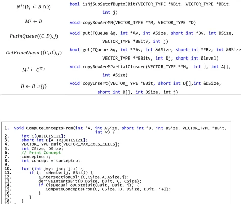
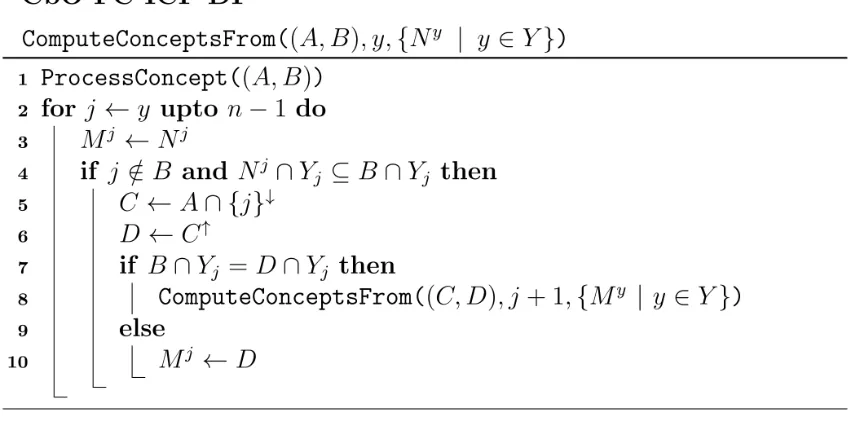
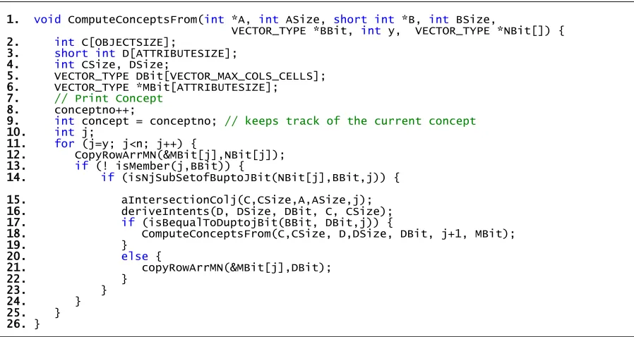
FIGURE5.6,ALGORITHM5.4–COMPUTECONCEPTSFROM–PARALLEL-IN-CLOSE3 ... 81

FIGURE5.7,COMBINEDDEPTHANDBREADTHFIRSTRECURSIVECALLTREE ... 82

FIGURE5.8,ALGORITHM5.5-DIRECTPARALLELIN-CLOSE3(THEDASHLINESSHOW THEDIFFERENCEWITHFIGURE5.6) ... 83

FIGURE5.9,ALGORITHM5.6-QUEUEPARALLELIN-CLOSE3,(DASHEDLINESHIGHLIGHT THEDIFFERENCESWITHFIGURE5.8) ... 84

FIGURE5.10,DIRECTPARALLELIN-CLOSE3 ... 87

FIGURE5.11,SIMPLEQUEUEPARALLELIN-CLOSE3 ... 87

FIGURE5.12,OPENMPPARALLELIN-CLOSE3 ... 88

FIGURE5.13,(A)MUSHROOM,(B)AD, (C)ADULT,(D)T1014D100K(E)M10X30G120K DATASETVSLEVELSFORPARALLELIN-CLOSE3ALGORITHMS ... 89

FIGURE5.14,TIMEVSDENSITYFORLEVEL=2,CORES-12 ... 90

FIGURE5.15,TIMEVSOBJECTSFORLEVEL=2,CORES-12 ... 90

FIGURE5.16,ATTRIBUTESVSTIMEFORLEVEL=2,CORES-12 ... 91

FIGURE5.17,STRUCTUREOFSCRACTHPADUSEDTOSTORECONCEPTSGENERTED ... 94

FIGURE5.18,SAMPLEVALUESOFSCRATCHPAD ... 94

FIGURE5.19,OPENMPINITIALPARALLELIZATIONCODEUSEDTOCALLRECURSIVE FUNCTIONFROMMAINPROGRAM ... 96

FIGURE5.20, RECURSIVECALLFROMNAIVEPARALLELIN-CLOSE3IMPLEMENTATION ... 96

FIGURE5.21,DIRECTLYSPAWNINGPARALLELTASKSINDIRECTPARALLELIN-CLOSE3 IMPLEMENTATION ... 97

FIGURE5.22,GENERATINGPARALLELTASKSINQUEUEPARALLELIN-CLOSE3 ALGORITHMS ... 98

FIGURE5.23,SPAWNINGPARALLELTASKSINSIMPLEQUEUEPARALLELIN-CLOSE3 IMPLEMENTATION ... 99

FIGURE5.24,SPAWNINGPARALLELTASKSINOPENMPQUEUEPARALLELIN-CLOSE3 IMPLEMENTATION ... 99

FIGURE5.25,HOTSPOTANALYSISOFTHESERIALINCLOSE3,AINTERSECTIONCOLJ() FUNCTION ... 100

FIGURE6.1,DISTRIBUTEDMEMORYSYSTEM(P.PACHECO,2011) ... 103

FIGURE6.2,CLUSTERCOMPUTERARCHITECTURE (SILVA&BUYYA,1999) ... 104

FIGURE6.3,ACLUSTERCOMPUTINGSYSTEMARCHITECTURE(HUSSAINETAL.,2013) ... 105

FIGURE6.4,MASTERWORKERPATTERN(MATTSON,SANDERS,&MASSINGILL,2004) ... 107

xii

FIGURE6.6(A),PSEUDOCODE-PART-I-DISTRIBUTEDMEMORYPARALLELIN-CLOSE3 ... 111

FIGURE6.6(B),PSEUDOCODE-PART-II-DISTRIBUTEDMEMORYPARALLELIN-CLOSE3 .... 111

FIGURE6.7,USERDEFINEDTYPEREPRESENTINGTHERECURSIVEALGORITHM PARAMETERS ... 113

FIGURE6.8,WORKERCOMPUTECONCEPTSFROM()FUNCTIONPROTOTYPE ... 113

FIGURE6.9,SENDMESSAGETOWORKER()FUNCTION ... 114

FIGURE6.10,RECEIVEPAYLOAD()FUNCTION ... 114

1

1

I

NTRODUCTION

1.1 Introduction

There is a huge amount of raw data that is produced each day. Since this raw data cannot be used as it is, knowledge in form of structures or patterns needs to be extracted from the data. This extraction of knowledge from data is known as data mining, and data analysis is the term used for further analysis and transformation of the structures found (Poelmans, Elzinga, Viaene, & Dedene, 2010; Poelmans, Ignatov, Kuznetsov, & Dedene, 2013a; Wille, 2002).

2

and biology (Andrews, 2015; Poelmans et al., 2010; Poelmans, Ignatov, Kuznetsov, & Dedene, 2013b; Tilley, Cole, Becker, & Eklund, 2005).

In order to define the complexity of the algorithms that generate formal concepts a brief introduction of the terms are described in this chapter, these are formally covered in depth in Chapter 3 of the thesis. In Formal Concept Analysis, a formal context is defined as a set of structure K = (G, M, I) where G and M are sets representing all the objects and attributes respectively for a given dataset. I represent a binary relationship between G and M. All the generated concepts of a context can be represented in a Lattice represented by L. Then the total number of concepts can be represented by |L|. If we consider |G| to be the number of objects in a given dataset, then number of concepts is at most 2|G|_{. The time complexity of generating} all concepts is in general a polynomial function with respect to the number of objects (Hitzler & Schärfe, 2009). For example, Kuznetsov’s CbO algorithm has a time complexity of O(|G|2_{|M||L|) and is therefore computationally time consuming. Here |M| represents the} number of attributes in the given context (Kuznetsov & Obiedkov, 2002). This is significant for large datasets having millions of objects. Hence there is a need for faster algorithms that are able to tackle large datasets (Old & Priss, 2004).

Classical FCA algorithms for example Chein, NextClosure, Norris, Bordat were only capable of handling smaller datasets running upto only thousands of objects (Bordat, 1986; Chein, 1969; Ganter, 1984; Norris, 1978). There have been numerous attempts to build upon the classical FCA algorithms. Recent algorithms such as AddIntent, Berry, FCbO and the In-Close family of algorithms, improve upon the classical algorithms (Andrews, 2009, 2015; Berry, Bordat, & Sigayret, 2007; Outrata & Vychodil, 2012; van der Merwe, Obiedkov, & Kourie, 2004).

3

1.2 Research Questions

The fundamental research question this thesis addresses is: what is the best parallel solution for computing formal concepts? Is there a parallel solution that outperforms all other parallel and serial solutions? The most important feature of performance is the speed of computation, but factors such as scalability should also be considered. It may be that the ‘best’ solution involves some compromise between speed, scalability and memory requirements. Clearly, an exhaustive comparison of all solutions is beyond the scope of this work, but a sufficient answer to the research question will be provided by defining and examining a representative subset of all solutions.

The fundamental research question will be answered by answering the following sub-questions:

1) What is the most appropriate existing serial algorithm to choose for parallelization? This may simply be the most efficient serial algorithm, but it is possible that some algorithms are not suitable for parallelization and appropriateness should also consider scalability and memory requirements.

2) What are the options for parallelizing the chosen serial algorithm (e.g. shared memory, distributed solutions) and which options may be the best in terms of speed and scalability?

3) How do parallel versions of the chosen serial algorithm compare with each other and with existing parallel solutions?

These three questions are answered in the thesis and a guide on where these questions are addressed are given in Section 1.3

1.3 Objectives and Structure of the Thesis

4

The second sub question on parallelizing the chosen serial algorithm is answered in Chapter 5 and Chapter 6. These two chapters present detail descriptions of new, shared memory and distributed memory parallel FCA algorithms. The parallel algorithms presented in this thesis are parallel variants of the fastest serial FCA algorithm. Several researches have concluded through empirical testing that the CbO family of algorithms provides the best performance (Andrews, 2009, 2011, 2015, Krajca et al., 2008, 2010a; Outrata & Vychodil, 2012; Strok & Neznanov, 2010). The first sub question on identifying the best serial algorithm is presented in detail in Chapter 4. This chapter describes the comparison of eight different variants of the CbO algorithm in a level playing field. The algorithms, which highlight the key features found in contemporary CbO based algorithms, are presented using the same pseudocode notation, and implemented from the pseudocode notation in the same way. The fastest serial FCA algorithm selected by analytical and empirical comparison was selected as the algorithm to be parallelised. The final sub question on the comparison of the parallel versions is addressed in Chapter 5 and Chapter 6. Here the implementations of the new parallel algorithms are compared with their serial counterparts and other parallel implementations.

1.3.1

Methodology

Details of the methodology used in this research is presented in Chapter 2. This include details of how key serial FCA algorithms were compared, and the evaluation and comparison of the new parallel algorithms presented in this thesis.

1.3.2

Formal Concept Analysis

A background to formal concept analysis is presented in Chapter 3. Many serial algorithms generate all the formal concepts of a given context. The limitations of serial formal concept analysis algorithms are presented in Section 3.3. A brief summary of existing parallel algorithms is presented in Section 3.4. The rational for developing parallel formal concept analysis algorithms and the research work carried out is also presented in Chapter 3.

1.3.3

Comparison of existing serial algorithms

5

according to several researchers. The eight variations highlight the three key features that are prominent in recently developed CbO algorithms (FCbO, In-Close, In-Close II, In-Close III). The fastest serial FCA algorithm found in this analysis was selected as the candidate algorithm for parallelization efforts. The selected algorithm was also checked to ensure that it was suitable for parallelization. To validate that the fastest serial algorithm produces the best performance, two other serial algorithms that were considered were also parallelized and their results compared.

1.3.4

Shared Memory Parallel Algorithms

Modern computers are shared memory parallel machines with multiple cores. A program that fully utilizes the modern computer hardware has to be explicitly programmed using a shared memory programming framework. Chapter 5, presents three new shared memory FCA algorithms that parallelize the best serial FCA algorithm found in Chapter 4. These algorithms were implemented in C++ using the OpenMP shared memory framework. A detail empirical comparison of several additional parallel algorithms that are based on key serial algorithms presented in Chapter 4 is also made. Finally, this chapter presents optimization strategies used in the parallel implementation.

1.3.5

Distributed Memory Parallel Algorithms

Shared memory machines have limitations when it comes to scaling. Clusters that consist of several independent computers connected through a high bandwidth network are commonly used to build powerful parallel machines. Clusters, which are scalable parallel computers, are essentially distributed memory computing machines with each computer (node) in the cluster having its own private memory. Distributed parallel algorithms typically use message passing between computing nodes to coordinate parallel computation. A new distributed parallel FCA algorithm and its implementation is presented in Chapter 6. This parallel algorithm is also based on the fastest serial FCA algorithm selected from Chapter 4.

1.4 New FCA algorithms presented in this Thesis

6

of the three enhancements used in modern CbO based FCA algorithms. The three algorithms are the CbO Full Closure Combined Depth First and Breadth First Search Algorithm (CbO-FC-DBF), CbO Full Closure Inherited Canonicity Test Failure and Depth First Search Algorithm (CbO-FC-ICF-DF) and the CbO Partial Closure Inherited Canonicity Test Failure and Depth First Search Algorithm (CbO-PC-ICF-DF). The algorithms are summarized in Table 1.1, in the order they are presented in the thesis.

Table 1.1, List of new algorithms presented in the thesis

New Algorithm Type of Algorithm Presented In

CbO-FC-DBF Serial Figure 4.6

CbO-FC-ICF-DF Serial Figure 4.8

CbO-PC-ICF-DF Serial Figure 4.11

7

2.

METHODOLOGY

2.1

Introduction

This research involved developing new algorithms and optimizing existing algorithms that can generate formal concepts for large data sets. This required a systematic methodology in initially identifying the best serial candidate algorithms which exist. The selected algorithms were taken forward into making parallel versions. At the end of the research, the performance of these newly modified algorithms, were systematically compared with existing algorithms.

The comparison of the efficiencies of different algorithms needed to be conducted at both the theoretical and practical level (Balakirsky & Kramer, 2004).

8

To compare different algorithms practically, carefully designed experiments needed to be carried out to test the running time of actual programs that implement these algorithms (Balakirsky & Kramer, 2004).

The experimental research methodology was used in this research to practically compare the different algorithms considered and presented. This methodology is the basis of the scientific method where the researcher manipulates one or more variables, and controls and measures any changes in other variables (Kumary, 2005; Ross, Morrison, & Mahwah, 2004). Here a series of carefully controlled experiments were designed and conducted. Andrews, 2015; Krajca, Outrata, & Vychodil, 2010; Kuznetsov & Obiedkov, 2002; Outrata, 2015; Strok & Neznanov, 2010 have all used a similar approach to compare actual programs that implement a set of algorithms.

Here the dependent variable time was measured varying each one of the independent variables, the number of objects, the number of intents and the density of a context while keeping the other two independent variables fixed.

2.2

Method of Sampling

The basic technique used for measuring time in a computer system is similar to how a stop watch can be used to measure a running experiment (Lilja, 2005). A computer system has an internal counter that measures the number of clock ticks from the time the computer was switched on. To measure the time taken for an experiment to run, the researcher would have to use a library function that would return the number of clock ticks. The difference of two measurements one taken one at the beginning and the second at the end of the experiment is the number of clock ticks taken for the experiment. This can be then converted using another library function to a wall clock time (Lilja, 2005).

A program’s execution time is non deterministic, hence the measurement needs to be taken multiple times. It is misleading to represent the summary of multiple readings using a single statistical value such as the mean or the median. Appropriate statistical rigor is needed to ensure that the measurements can be relied upon to infer a decision regarding the different algorithms that are measured. This includes identification and removal of outliers.

9 1. Experimental Mistake

2. Random Errors

Care was taken to avoid experimental mistakes by double checking the exact part of the code that needed to be measured was consistent across the different programs. The algorithms were implemented using common code blocks which ensured that all the programs considered were written in a similar level of complexity and represented the high-level logic of the algorithms that they represented.

Random errors on the other hand are completely non-deterministic and needs to be handled using a statistical approach. These could be due to the result random processes within the system at both hardware and software level.

Vladimirov had noted that the first run of a program is slower than its subsequent runs. In the experiments carried by Colfax the first three timing results were ignored to eliminate this known outlier (Vladimirov, Asai, & Karpusenko, 2015). In this research every experiment was measured 13 times, the first 3 sample reading were ignored as outliers. The remaining 10 sample reading was used to represent the timing of running the program.

Total Program Execution time = ,1 + ,2 + ,3

Where

,1 = Time taken to read sample data set

,2 = Time taken to execute the algorithm

,3 = Time taken to store and display the results

Both ,1 and ,3 required Input/Output from secondary storage devices but was the same across all algorithms for a given dataset. To further eliminate potential random errors due to Input/Output only ,2 was measured for all programs. Instrumented code was placed in the main program just before and after the function call to execute the complete algorithm.

10

Table 2.1, Statistical Analysis carried out for one raw experimental result

Dataset : Mushroom - Algorithm : CbO.PC.DBF (In-Close 2)

Sample Concepts Time

1 226921 0.9184910

2 226921 0.8537550

3 226921 0.8541490

4 226921 0.8537010

5 226921 0.8534310

6 226921 0.8540500

7 226921 0.8534830

8 226921 0.8534220

9 226921 0.8539590

10 226921 0.8536050

11 226921 0.8536480

12 226921 0.8539750

13 226921 0.8534100

mean 0.8536684

median 0.8536265

min 0.85341

max 0.85405

IQR 0.00067575

95% confidence error 0.000176484 Outlier Boundary 1 =

(Q1 - 1.5 x IQR) 0.85276825

Outlier Boundary 2 =

(Q3 – 1.5 x IQR) 0.85457025

Table 2.1 shows how statistical analysis was carried out for one single experimental reading. Raw readings are presented as timing in this Table. From the 95% confidence level from this sample we can conclude that the measurements in this specific instance is accurate to the first 3 decimal places. This specific sample was for the timing result ,2 for running the program representing the algorithm CbO-PC-DBF (In-Close2). The program was run 13 times, the first three results were excluded from the statistical analysis as outliers. We can clearly see in the above example that first reading is an outlier.

11

a T-Distribution. This was because the sample size was less than 30 (Georges, Buytaert, & Eeckhout, 2007)

The 95% confidence levels are shown in Tables that represent real datasets. One can observe that the experimental data cluster around the mean. This is because the programs were compiled and run using the C language which doesn’t require any runtime environment to execute the programs. In addition, the computer used for the experiment was a node in a cluster running a minimalistic Linux based operating system. The executable programs and the datasets were submitted to the computer using a login terminal node. The Colfax cluster which was used to run the system ensured that the computational nodes only ran the submitted program at a given point in time. This ensured that there were no side effects during the experiment due the execution of other background programs.

2.3

Statistical Significance of empirical results

2.3.1

Introduction

The one-way analysis of variance (one way Anova) and the t-Test for Two sample assuming unequal variances were used to show that the empirical results were statistically significant.

2.3.2

One-way analysis of variance

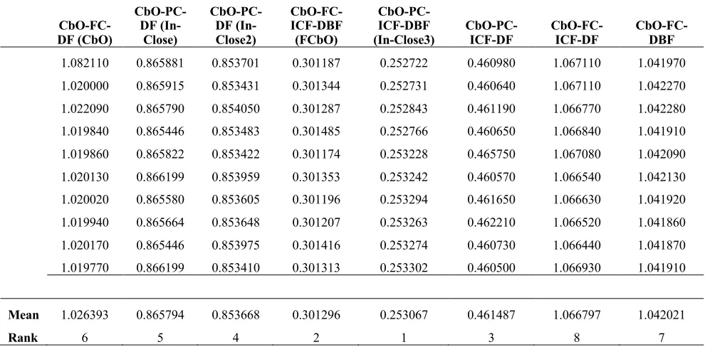
To demonstrate that the empirical timing results between the implemented algorithms were statistically significant Kruskal-Wallis one way analysis of variance (one way Anova) was used (Kruskal & Wallis, 1952). An example is provided to describe how this analysis was carried out. Table 2.2 contains the actual experimental data of the 10 sample runs for the mushroom dataset using the eight serial implementations of the algorithms described in Chapter 4 of the thesis.

The null hypothesis 1₂ assumes that means of experimental run time of all the implemented algorithms are the same. The alternative hypothesis is that there exists at least one mean which is different from another mean.

1₂: 4₅ = 4₇ = 4₈ = ⋯ = 4_:

12

Table 2.2, Empirical Timing (seconds) for each serial algorithm running the mushroom dataset

CbO-FC-DF (CbO)

CbO-PC-DF

(In-Close)

CbO-PC-DF (In-Close2)

CbO-FC-ICF-DBF

(FCbO)

CbO-PC-ICF-DBF (In-Close3)

CbO-PC-ICF-DF

CbO-FC-ICF-DF

CbO-FC-DBF 1.082110 0.865881 0.853701 0.301187 0.252722 0.460980 1.067110 1.041970 1.020000 0.865915 0.853431 0.301344 0.252731 0.460640 1.067110 1.042270 1.022090 0.865790 0.854050 0.301287 0.252843 0.461190 1.066770 1.042280 1.019840 0.865446 0.853483 0.301485 0.252766 0.460650 1.066840 1.041910 1.019860 0.865822 0.853422 0.301174 0.253228 0.465750 1.067080 1.042090 1.020130 0.866199 0.853959 0.301353 0.253242 0.460570 1.066540 1.042130 1.020020 0.865580 0.853605 0.301196 0.253294 0.461650 1.066630 1.041920 1.019940 0.865664 0.853648 0.301207 0.253263 0.462210 1.066520 1.041860 1.020170 0.865446 0.853975 0.301416 0.253274 0.460730 1.066440 1.041870 1.019770 0.866199 0.853410 0.301313 0.253302 0.460500 1.066930 1.041910

Mean 1.026393 0.865794 0.853668 0.301296 0.253067 0.461487 1.066797 1.042021

Rank 6 5 4 2 1 3 8 7

The one-way Anova which is also known as the single factor analysis of variance was carried out using Microsoft Excel. The output generated from the analysis using Excel is shown in Table 2.3 with the significance level set to 5%.

Table 2.3, One Way Analysis of variance (one way anova) for dataset in Table 2.2

SUMMARY

Groups Count Sum Average Variance

CbO-FC-DF 10 10.263930 1.026393 0.000383718

CbO-PC-DF 10 8.657942 0.865794 7.28848E-08

CbO-PC-DF 10 8.536684 0.853668 6.08649E-08

CbO-FC-ICF-DBF 10 3.012962 0.301296 1.11922E-08

CbO-PC-ICF-DBF 10 2.530665 0.253067 6.85845E-08

CbO-PC-ICF-DF 10 4.614870 0.461487 2.54153E-06

CbO-FC-ICF-DF 10 10.667970 1.066797 6.60456E-08

CbO-FC-DBF 10 10.420210 1.042021 2.57656E-08

ANOVA

Source of Variation SS df MS F P-value F crit

Between Groups (B) 8.156074 7 1.165153365 24112.95822 1.2384E-118 2.139655512

Within Groups (W) 0.003479 72 4.83206E-05

13

The Summary Section of Table 2.3 calculates the sum, average and variance of the experiment of the dataset presented in Table 2.2.

In the ANOVA section of Table 2.3 of the analysis the following definitions and formulae is used.

The sum of squares CC_B, CC_D, CC_E and CC_F are defined as follows.

CCB = G(H@B− H̅B)7 @

CC_D = G G(H_@B @

− H̅)7 B

CC_E = G G(H_@B @

− H̅_B)7 B

CC_F = G K_B(H_@B − H̅_B)7 L

Where Kis the sample size of jth _{sample, H̅}

Bis the mean of the jth group sample and H̅is the mean

of the entire sample.

n is defined as follows.

K = G K_B M

BN5

Where Ois the number of samples.

The degrees of freedom PQD, PQFand PQEare defined as follows.

PQD = K − 1

PQ_F = O − 1

PQE = G(K − 1) M

BN5

14 The mean square is defined as follows.

*C = CC/PQ

The mean square *C_D, *C_F and *C_E are defined as follows.

*C_D = CC_D/PQ_D

*C_F = CC_F/PQ_F

*C_E = CC_E/PQ_E

The S value is defined as follows.

S = _*C*CF E

The T_UVWXY for the (right tailed) F probability distribution for two data can be computed using the SZ=[\]=^_\=`K() function which requires S, PQFand PQEas parameters.

TUVWXY = SZ=[\]=^_\=`K(S, PQF, PQE)

The S_ab@cvalue is the inverse of the (right tailed) F probability distribution and can be obtained using the SdKef][f() function which requires g, PQ_Fand PQ_E as parameters.

S_ab@c = SdKef][f(g, PQ_F, PQ_E)

Here gis the significance level.

We can reject the null hypothesis 1₂ if S > S_ab@c and T_UVWXY < g

2.3.3

t-Test for Two sample assuming unequal variances

To show that the empirical timing results obtained for the two algorithms which needed to be compared has statistical significance the t-Test for two sample assuming unequal variances (Boslaugh, 2012) was used. In most cases the comparison was between the two algorithms that produced the best results. It was also used to compare the newly developed parallel algorithms with existing parallel algorithms.

The null hypothesis H0 assumes that the means of experimental run time of both the

implemented algorithms are the same. The alternative hypothesis is that there is a statistically significant difference between the two sample means that are considered.

15 12: 45 = 47

1_;: 4_@ ≠ 4₇

Table 2.4, shows the output of the Excel analysis of the t-Test for the timing results of the In- Close3 and FCbO algorithms from Table 2.2.

Table 2.4, t-Test: Two-Sample Assuming Unequal Variances for the two fastest algorithms (Rank 1 and Rank 2 in Table 2.2) In-Close3 and FCbO

CbO-PC-ICF-DBF (In-Close3)

CbO-FC-ICF-DBF

(FCbO)

Mean 0.2530665 0.3012962

Variance 6.85845E-08 1.11922E-08

Observations 10 10

Hypothesized Mean Difference 0

df 12

t Stat -539.9786481

P(T<=t) one-tail 5.47963E-28 t Critical one-tail 1.782287556 P(T<=t) two-tail 1.09593E-27 t Critical two-tail 2.17881283

The \_jcVcis calculated as follows. H̅₅and H̅₇ are the means of sample1 and sample2 respectively. K₅and K₇ are the sample size for sample1 and sample2 respectively. [₅ and [₇ represent the sample deviations.

\_jcVc = H̅5− H̅7

kl[57 K₅+[7

7 K₇m

The degrees of freedom PQ is calculated as follows.

PQ = l

[₅7 K5+

[₇7 K7m

7

1 K₅− 1 l[5

7

K₅m +K₇1− 1 l[7 7 K₇m

The T_cnopcV@W for the student’s T distribution can be found by using the T ,Z=[\]=^_\=`K() function which requires \jcVc and PQ as parameters.

16

The \ab@c@aVW cnopcV@Wvalue is the inverse of the student’s T probability distribution and can be obtained using the ,dKef][f() function which requires gand PQas parameters.

\_{ab@c@aVW cnopcV@W} = ,dKef][f(g, PQ)

Here gis the significance level.

We can reject the null hypothesis 1₂ if |\jcVc| > \ab@c@aVW cnopcV@W and TcnopcV@W < g

2.4

Detail activities undertaken in this research

After the literature review was carried out, a set of potential serial algorithms were identified. Each serial algorithm was implemented in a similar manner, taking care that any difference in performance could be only due to algorithm design and not due to implementation details or different optimizations. Next, they were tested on a 'level playing field'. Test data was carefully selected and prepared so that the algorithms could be tested on a number of key independent parameters, such as context density, number of attributes and number of objects. Details of the tests carried out are described in Section 2.5

The experiments were designed to determine the best candidate algorithm/s to take forward for parallelization. Next code profiling was used to identify parts of the program that could be optimized further. This resulted in new algorithms that can efficiently handle large datasets.

17

2.5

Benchmarking of the implementations

Other research have reiterated the importance of having a set of publically available standard datasets for comparing FCA algorithms (Andrews, 2009; Kuznetsov & Obiedkov, 2002). Although there are no standard dataset established for testing FCA algorithms several research studies have used publicly available datasets for this purpose (Andrews, 2009, 2011, 2015; Frank & Asuncion, 2010; Krajca, Outrata, & Vychodil, 2008; Krajca et al., 2010; Strok & Neznanov, 2010). In this research several popular public datasets such as the mushroom dataset, adult dataset from the UCI learning repository were used.

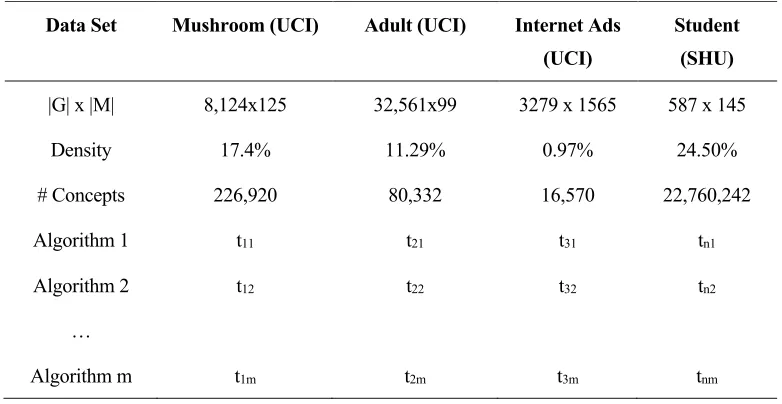
Table 2.5, shows how the performance of different algorithms for benchmarked datasets used in FCA literature would be depicted. In addition, random data experiments were also carried out.

Table 2.5, Sample test cases for actual datasets (timing in seconds)

A random dataset generator used in the FCA community was used to generate random datasets of particular characteristics. The generator can be used to generate a random dataset that matches the given number of objects, number of attributes and density. The generated dataset has a filename that indicates its characteristics. For instance, the random dataset n100m20000d5s1000.cxt has 100 attributes (n), 20,000 objects (m) and has a density of 5%. The number 1000 after the latter ‘s’ indicates the random generator seed used. The same generated dataset file was used in all experiments that required a dataset of 100 attributes, 20,000 objects with a density of 5%. The number of concepts that is there for a given dataset is dependent on the number of attributes, number of objects and the density. It is also dependent on the arrangement of crosses that are there in the dataset that represents the binary

Data Set Mushroom (UCI) Adult (UCI) Internet Ads

(UCI)

Student (SHU)

|G| x |M| 8,124x125 32,561x99 3279 x 1565 587 x 145

Density 17.4% 11.29% 0.97% 24.50%

# Concepts 226,920 80,332 16,570 22,760,242

Algorithm 1 t11 t21 t31 tn1

Algorithm 2 t12 t22 t32 tn2

…

18

incidence relationship between the number of objects and the number of attributes. In general, given a dataset of |G| number of objects the number of concepts at most would be 2|G|_.

The following large random datasets used in the FCA community was also used as benchmarking datasets. The M7X10G120K, M10X30G120K and the T10I4D100K datasets have the following characteristics (See Table 2.6). Here |G| and |M| represent the number of objects and the number of attributes respectively.

Table 2.6, Random Benchmarking datasets

Data Set M710G120K M10X30G120K T1014D100K

|G| x |M| 120,000 x 70 120,000 x 300 100,000 x1,000

Density 10.00% 03.33% 01.01%

# Concepts 1,166,343 4,570,498 2,347,376

2.6

Unit Testing the Implementations

All the implementations developed had a common core handling reading the dataset and generating an output file containing all the generated concepts.

The following datasets were used in order to unit test the implementations. Sample Dataset (Andrews, 2015), Tealady dataset, Water Lilies dataset (Ganter & Wille, 1999), n100m100d5s1000.cxt, n200m100d5s1000.cxt and the mushroom. These datasets have 10, 65, 112, 395, 1,062, 226,921 concepts respectively. The output file generated from the implementations were compared using the diff utility with the output file generated by an open source implementation of InClose1 _{for each of the datasets. If there was any deviation noted}

in diff it was assumed that the unit test had failed. In a majority of cases the difficulty was to get the implementation to pass the simpler datasets upto Water Lilies. Later once the artificial dataset unit tests were passed, the implementations usually passed the mushroom real-world dataset without any modification. This approach was used to test all the serial, shared memory parallel and the distributed parallel algorithm implementations.

2.7

Comparison of Serial Implementations of FCA

19

Kuznetsov and Obedkov (2001). Andrews (2014) re-specification of the algorithms are described in the same level of abstraction. Each of the different code blocks used in the eight CbO algorithms were implemented as C++ functions. The eight algorithms had 17 unique code blocks which were implemented as 16 separate C++ functions. (Two code blocks mapped into one C++ function.) The algorithms were finally implemented in C++ by assembling the C++ functions developed. The algorithms were implemented in an un-optimized way to focus on the comparison of the algorithms themselves and not on any efficiencies provided by optimizing the code. All implementations used the same data structures for representing objects, attributes and the context. The details of the different data structures used are given in Table 4.2, Kuznetsov and Obedkov (2001) also raised the importance of using similar data structures when comparing different algorithms.

The eight algorithms were implemented in an un-optimized way. An un-optimized implementation of an algorithm is also a very good starting point for subsequent optimization and parallelization. Knuth (1974) famously said that premature optimization is the root of all evil. Jackson (1975) has also cautioned against early optimization which can result in a design that is not as clean as it could have been or code that is not correct, as a result of the complicated code due to the optimizations carried out.

The approach used to implement the eight algorithms using common code blocks ensured that the programs correlated to the algorithms in a similar way. Empirical testing was carried out on the code compiled with the Linux Intel C++ Compiler version 15. The implemented algorithms were tested on Intel ® AI Cloud2 _{running in a Colfax Cluster}3 _{on a Compute Node}

20

and 5% respectively (See Table 4.7), All the programs used in comparing the serial implementations were compiled in debug mode with no optimization (compiled using the Intel Compiler flags –O0 –g) to ensure that the compiled code represented a true reflection of the high level algorithms that were compared. To verify that the computer and compiler used for the experiments had no side effect in the results the three real world datasets were tested again on three other computers (an Intel Core i5-5210M CPU @ 2.5GHz, with 8GB RAM, running a Microsoft Windows 7 - 64 bit operating system and a Core i7-4650U CPU @ 3.3GHz with 8GB RAM running Microsoft Windows 8 – 64 bit operating system) with two windows compilers (Microsoft Visual Studio 2010 and Intel C++ Compiler version 16). Each machine ran each of the programs compiled by both the Intel and the Microsoft compilers. The experiments were also executed on the Archer Super Computer which has a node consisting of two two 2.7 GHz, 12-core Intel ® Xeon ® E5-2697 v2 processors with 64GB RAM each. A Cray compiler was used for the compilation. The results obtained had the same variation as the results shown in Section 4.4.

2.8

Experimental Testing of Parallel Algorithms

The parallel algorithms that are proposed were experimentally validated and tested using a similar approach to the Serial programs. The scalability of parallel programs is represented by the following formulae.

C_q = ,5 ,_q

Where T1 is the time taken to execute a program in one processor and Tp the time taken to

execute a program on p number of processors. A graph can be used to show how scalable the implementation is.

Here too all samples were statistically analysed as mentioned in Section 2.2.

The OpenMP shared memory implementations were tested using the Intel ® AI Cloud mentioned in Section 2.7

21

topology four compute nodes are connected to each Aries router; 188 nodes are grouped into a cabinet; and two cabinets make up a group. (Turner & McIntosh-Smith, 2017). By nature a super computer provides dedicated access of the compute nodes required to run a program. This ensures that during the empirical testing that all the test results reflects only the execution time of the programs that were run.

_________________________________________

1 _{https://sourceforge.net/projects/inclose/} 2 _{https://ai.intel.com/devcloud/}

22

3.

FORMAL CONCEPT ANALYSIS

3.1 Formal Concept Analysis Background

Knowledge Representation is the field in artificial intelligence which focuses on the representation of information, that can be used by a computer to solve complex problems. Ontologies, which capture the relationships between concepts is a knowledge representation technique. Ontologies are generally created by domain experts (Uschold & Gruninger, 1996). There are significant advantages if ontologies can be created automatically from structured data (Alani et al., 2003). A form of clustering algorithms called biclustering algorithms can be essentially used for this purpose. Clustering is the task of grouping related sets of data together (Kaytoue, Kuznetsov, & Napoli, 2011). Even in situations where the clustering algorithms are only able to capture simpler relationships such as an is-a relationship, this still has significant practical applications in many domains.

Formal Concept Analysis can be thought of as a form of biclustering which can generate is-a relationships from structured binary tabular data. The is-a relationship forms the basis of grouping concepts into super concepts and sub concepts and is represented as a concept lattice. Implications and Associate Rules are direct by products of a concept lattice (Wille, 2005b).

23

in the “classical theory of concepts” are mathematically represented as formal concepts in formal concept analysis (FCA). In psychology/philosophy concepts are formally definable by its features. This approach is still a popular way to represent concepts although the “classical theory of concepts” doesn’t accurately represent human cognition. The concepts found in FCA are called “formal concepts” to avoid confusion non-mathematical definition of concepts(Priss, 2006).

Knowledge is represented in formal concept analysis as a formal context. This describes a binary relationship between a set of objects and a set of attributes of a domain.

A precise definition of a formal context is given below.

A formal context is defined as ! ∶= (%, ', ()

Where % is a set of objects, ' a set of attributes and ( a binary incidence relationship between

G and ' with ( ⊆ % × '.

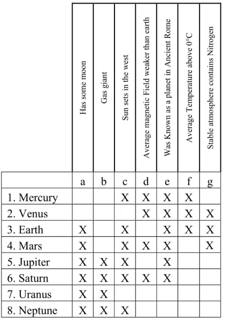
Since formal contexts are a binary relationship, they can be represented as cross tables. Here each object and attribute is represented as a row and a column respectively (Ganter, Stumme, & Wille, 2002; Wille, 1982).

24

rows are known as objects and the columns are known as attributes. A formal concept is defined as a pair of maximum of a set of objects and a set of attributes. For the earlier example

Figure 3.1, A Formal context about planets in our solar system (Krötzsch & Bernhard, 2009)

25

of this formal concept and the attribute form the intent. A mathematical definition of Formal Concepts is given below.

For a set of objects - ⊆ % the set -¢ is defined as

-._{∶= {0 ∈ ' | 0 ( 3 for all 3 ∈ -}}

Similarly for a set of attributes : ⊆ % the set :¢ is defined as

:._{∶= {3 ∈ % | 0 ( 3}

for all

(-, :) is a formal concept if -′ = : and :′ = -.

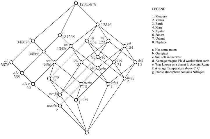
There are many formal concepts in a formal context. All the possible formal concepts that are there in a formal context can be generated and be represented in a concept hierarchy. A concept lattice can be used to represent a concept hierarchy (See Figure 3.2).

26

Here the object and attribute indices 1 to 8 and a to g are used for brevity. The two examples mentioned earlier map to the concepts ({5,6,7,8},{a,b}) and ({3,4,5,6,7,8},{a}) respectively in the Lattice. They are the left most vertex of the lattice and the vertex immediately above. In the example taken the concept ({Earth, Mars, Jupiter, Saturn, Uranus, Neptune}, {Has some Moon})(Shown as ({3,4,5,6,7,8},{a}) in lattice) is the sub concept of ({Jupiter, Saturn, Uranus, Neptune}, {Gas Giant, Has Some Moon}) (Shown as ({5,6,7,8},{a,b} in lattice). Accordingly in the concept lattice the concept ({3,4,5,6,7,8},{a}) is above the concept ({5,6,7,8},{a,b}) as it is more general. A mathematical definition of the relationships between formal concepts is given below.

Let ! ∶= (%, ', () define a formal context. Assuming (-<, :<) and (-=, :=) are formal

concepts of !.

(-_<, :_<) ≤ (-₌, :₌) ∶= -_< ⊆ -₌(⟺ :_< ⊇ :₌)

(-<, :<) is called the sub concept of (-=, :=), and (-=, :=) is called the super concept of

(-_<, :_<). In the Concept Lattice the more general concepts are above and the specific concepts are below. The set of all formal concepts of ! together with the defined order relation is denoted by A(%, ', (), which can be represented as a Concept Lattice (See Figure 3.2)

27

described in the development of interactive museum applications for searching virtual objects and physically navigating museum exhibits by Wray and Eklund (Wray & Eklund, 2011, 2014).

3.2 FCA Algorithms

There are several well-known algorithms that generate a set of all the formal concepts that are there in a formal context. The number of concepts is known to be exponential of the size of the input context (Kuznetsov & Obiedkov, 2002). Algorithms that generate formal concepts broadly fall into two categories

(a) Generate only the list of concepts (b) Generate a concept lattice.

Kuznetsov compares the efficiency of ten algorithms that generate formal concepts (Kuznetsov & Obiedkov, 2002). Some of the algorithms compared included NextClosure (Ganter, 1984), Bordat (Bordat, 1986), Close by One (Kuznetsov & Obiedkov, 2002), Lindig (Lindig, 2000), Chein (Chein, 1969), Nourine (Nourine & Raynaud, 1999), Godin (Godin, Missaoui, & Alaoui, 1995), Dowling (Dowling, 1993) and Titanic (Stumme, Taouil, Bastide, Pasquier, & Lakhal, 2000). Different algorithms use different strategies to generate a new intent. Some algorithms compute an intent explicitly by intersecting all the objects of the corresponding extent. Others intersect a generated intent with some object’s intent (Kuznetsov & Obiedkov, 2002).

A canonicity test is used by FCA algorithms to check if the current concept is being generated for the first time. In some of the algorithms complete closure of a concept is needed before the canonicity test, and in some the testing of the canonicity can take place before the complete closure (partial closure). Certain algorithms also keep track of the canonicity test failures which can be applied before closure (Andrews, 2015; Outrata & Vychodil, 2012).

28

algorithms that focus on this without computing the lattice (Outrata & Vychodil, 2012; Strok & Neznanov, 2010).

3.3 Limitations of Serial FCA Algorithms

Old and Priss have highlighted the need of developing algorithms that can handle large contexts (Old & Priss, 2004). There is no formal definition of what a large context is, however based on recent benchmarks a large context can be taken as consisting of over 100,000 objects and over 100 attributes resulting in millions of concepts (Andrews, 2017; Outrata, 2015). In real world datasets the size of attributes are limited in size. There is an explosion of data that is produced daily. In 2012, a study carried out by IBM estimated that 2.5 exabytes of data are produced daily (Wall, 2014). Structured data is still a significant type of data that is used in organizations (Desiere, 2015). FCA has been extended into areas such as data mining, web mining which involves large data sets (Fu & Nguifo, 2004). Datasets in domains such as genomics, internet of things, log analysis are significantly large and are growing at a rapid pace. For instance Genomics dataset sizes have been doubling every 18 months (Langmead & Nellore, 2018). There is a necessity for FCA algorithms to handle this volume of data. The possession of a fast algorithm for computing or updating the underlying concept lattice is an essential prerequisite in many applications for instance rule discovery, document ranking and program analysis (de Moraes, Dias, Freitas, & Zárate, 2016; Poelmans et al., 2013a, 2013b).

All computing devices used today are parallel machines. The introduction of multicore processors commenced around the year 2004 to solve the so-called power wall problem (See

Figure 3.3). Prior to this CPU manufacturers resorted to increase the clock speed of each new generation of CPU eventually reaching the critical power consumption of 130 Watts around 2004. Beyond this point, it was not economically possible to dissipate the heat produced by the CPU’s. Over the last decade CPU manufacturers have kept the clock speed and core size of a CPU as constants and have resorted instead to add extra cores to a single die in the CPU to get better performance (Chappell & Stokes, 2012).

29

of a modern computer needs to be a parallel algorithm. With the rapid increase of datasets that require analysis, the next generation FCA algorithms should be parallel in nature.

Figure 3.3, Processor/coprocessor core/thread parallelism (log scale) (Jeffers, Reinders, & Sodani, 2016)

3.4 Existing Parallel FCA Algorithms

Huaiguo Fu had created a parallel implementation of the NextClosure algorithm but it was limited to 50 attributes (Fu & Nguifo, 2004) this was subsequently greatly extended (Fu & Foghlu, 2008). Krajca (Krajca, Outrata, & Vychodil, 2008) presented a parallel algorithm called PFCbO which parallelizes the FCbO algorithm. This is also a variation of the CbO algorithm (Kuznetsov & Obiedkov, 2002). Krajca has also presented a distributed version of this algorithm that uses the Map Reduce distributed framework (Krajca & Vychodil, 2009).

The main contribution of the thesis are the new parallel FCA algorithms for shared memory and distributed memory models which are presented in Chapter 5 and Chapter 6 respectively.

T

hr

ea

ds

/C

or

es

30

4.

COMPARISION

OF

FCA

SERIAL

ALGORITHMS

4.1 Existing FCA Algorithms

Many of the classical algorithms such as Bordat, NextClosure, Chein, Lindig and Nourine are batch algorithms. These algorithms generate the entire context from scratch. Some of the other algorithms including Godin, Downling, Norris, Close by One (CbO), Kracja and In-Close are incremental algorithms. Incremental algorithms produces the concept set for the first ith

concepts at the ith _{step.(Chang-Sheng, Jing, Hai-Long, Long-chang, & Bing-ru, 2013; Gajdoš}

& Snášel, 2014; Sarmah et al., 2015).

31

Algorithms are described by their authors at different levels of abstraction. Some algorithms such as CbO are described by Kuznetsov using an abstract mathematical set notation (Kuznetsov & Obiedkov, 2002), while others such as FCbO (Outrata & Vychodil, 2012) or In-close (Andrews, 2009) are described in pseudo code which is In-closer to the implementation level in a programming language. Algorithms which are described in a higher abstract notation would be interpreted subjectively when other researchers implement them. A proper comparison of a set of algorithms can be carried out if they are described at the same level of abstraction. Andrews (2014) presents the five variations of the CbO algorithms using the same level of abstraction. In order to highlight the effects of the key features used in recent variations of the CbO algorithm this thesis introduces three new variations of the CbO algorithm presented using the same notation used by Andrews. They are the CbO full closure using a combined depth first and breadth first search (CbO-FC-BDF), CbO full closure using inherited canonicity test failures and depth first search (CbO-FC-ICF-DF), and CbO partial closure with incremental closing of intents using inherited canonicity test failures and depth first search (CbO-PC-ICF-DF).

This chapter presents the detail comparison of the three main enhancements that have been applied to Kusnotsov’s CbO algorithm. The three main enhancements considered are the partial closure with incremental closure of intents, inherited canonicity test failures and using a combined depth first and breadth first search. Eight variations of the CbO algorithm are presented and implemented in an un-optimised way allowing the identification of the best algorithms to select for future algorithmic enhancement such as parallelization.

32

Table 4.1 highlight the summary of the eight CbO variants presented in this paper. CbO-FC-DF is the base algorithm used, the rest are carefully selected variants that highlight the three key enhancements used.

Table 4.1, Eight Variations of CbO

Algorithm Originally Described in Use of a Queue Partial Closures failed canonicity Inheritance of tests.

CbO-FC-DF Krajca (Vychodil, 2008)

CbO-PC-DF In-Close (Andrews, 2009) X

CbO-FC-DBF New X

CbO-PC-DBF In-Close2 (Andrews, 2011) X X

CbO-FC-ICF-DF New X

CbO-PC-ICF-DF New X X

CbO-FC-ICF-DBF FCbO (Krajca, Outrata, & _{Vychodil, 2010)} X X

CbO-PC-ICF-DBF In-Close3 (Andrews, 2014) X X X

The algorithms have been named making use of the following abbreviations FC – full closure, PC – partial closure with incremental closure of attributes, DF – depth first search, DBF – combined depth and breadth search and ICF – inherited canonicity test failure. Algorithms that use the combined depth and breadth search feature (DBF) make use of a queue data structure.

33

4.2 Details of the Eight CbO based Algorithms

CbO-FC-DF (CbO – Full Closure, Depth First Search Algorithm)

Figure 4.1, CbO-FC-DF (CbO) algorithm pseudo code (Vychodil, 2008)

The CbO-FC-DF (CbO – Full Closure, Depth First Search) algorithm shown in Figure 4.1, was originally described by Vychodil (2008). In our discussion we will use this as our base algorithms. Here (", $) is the concept generated where " is the extent and $ is the intent. & is the number of attributes in the context and ' is the attribute that is currently being considered. The algorithm is invoked with (", $) = (*, *↑_{). Where * represents a complete set of extents.} Recalculation of already computed concepts can be avoided by the statements in line 3 and line 6.

, ∉ $

, ∉ $ enables skipping attributes in the current intent (Vychodil, 2008). Here if the currently considered attribute , is already a member of the currently considered intent then the extent of this has already been computed. This is due to the following observation.

{0,1,2, , , 2, , &}

= {0,1,2, , , 2, , &}

∩ {2}

The canonicity test is defined by the condition given in line 6.

34

Here 67 is a set containing all the attributes upto attribute ,. Due to the lexical order of

computing the concepts, the above condition becomes false only if 8 is lexically before $.

Thus it implies that the concept has been computed before and can be skipped. The extents and the intents are computed in line 4 and 5 respectively. A full closure is used in calculating the intent in line 5.

8 ← :

The complexity of CbO family of algorithms are ;(|=|>_{. |@|) (Kuznetsov & Obiedkov, 2002).} The implementation of CbO is given in Figure 4.2 to illustrate how the common code blocks are used in the actual algorithm implementation. Lines 2 to 8 of the implementation of DF contain declaration of variables. Lines 10 to 19 directly correspond to the CbO-FC-DF algorithm given in Figure 4.1. Table 4.2, shows details of the 17 code blocks used in the algorithms and their corresponding C++ functions used in the implementation. The

VECTOR_TYPE used in the code is a macro representing an unsigned 64 bit integer which is used

to store binary values.

Table 4.2, List of Functions used to implement the common code blocks

Code Blocks Common Function used in Implementation of the five algorithms

, ∉ $ bool isMember(int j, VECTOR_TYPE *BBit)

: ← " ∪ {,}↓

void aIntersectionColj(int **C,int &CSize,int *A ,int ASize,int j)

8 ← :↑ void deriveIntentsBit(short int **B, int &BSize, VECTOR_TYPE *BBit,

int *A, int ASize)

$ ∩ 67= 8 ∩ 67 bool isBequalToDuptojBit(VECTOR_TYPE *BBit, VECTOR_TYPE *DBit, int j)

" = : _{bool isEqual(int I1[],int I1Size,int I2[], int I2Size)}

$ ← $ ∪ {,} _{void insert(VECTOR_TYPE *BBit, short int B[], int &BSize, int j)}

$ = :↑B_C bool buptoJisEqualtoPartialClosureOfCuptoJBit(VECTOR_TYPE *BBit,

int C[], int CSize, int j)int C[], int CSize, int j)

$ ∩ 67= :↑BC bool buptoJisEqualtoPartialClosureOfCuptoJBit2(VECTOR_TYPE *BBit,

int C[], int CSize, int j)

DEFG&HEIEI(:, ,) _{void put(TQueue &q, int *Av, int ASize, int BSize, int j)}

=IFJKLMHEIEI(:, ,) _{bool get(TQueue &q, int}