Research Article
Spherical Harmonics for Surface Parametrisation
and Remeshing
Caitlin R. Nortje, Wil O. C. Ward, Bartosz P. Neuman, and Li Bai
School of Computer Science, The University of Nottingham, Jubilee Campus, Wollaton Road, Nottingham NG8 1BB, UK Correspondence should be addressed to Li Bai; [email protected]
Received 5 August 2015; Revised 2 November 2015; Accepted 9 November 2015 Academic Editor: Masoud Hajarian
Copyright © 2015 Caitlin R. Nortje et al. This is an open access article distributed under the Creative Commons Attribution License, which permits unrestricted use, distribution, and reproduction in any medium, provided the original work is properly cited.
This paper proposes a novel method for parametrisation and remeshing incomplete and irregular polygonal meshes. Spherical harmonics basis functions are used for parametrisation. This involves least squares fitting of spherical harmonics basis functions to the surface mesh. Tikhonov regularisation is then used to improve the parametrisation before remeshing the surface. Experiments show that the proposed techniques are effective for parametrising and remeshing polygonal meshes.
1. Introduction
Polygonal meshes are often used to represent the surfaces of graphical models. Often a mesh is irregular or unsatisfactory due to over- or undersampling or the triangularisation technique used. There is thus the need to improve the quality of the mesh by remeshing.
There are two main categories of remeshing techniques: parametrisation methods [1–5] and mesh adaptation strate-gies [6–8]. Parametrisation methods indirectly improve a given mesh by parametrising it, often through bijective mapping from the original mesh to a 2D planar domain. New sampling can then be performed on this planar domain and, using the inverse of the original mapping function, is mapped back to the surface to form a new mesh. Unlike parametrisation techniques, mesh adaption strategies directly improve meshes using relaxation or modification processes to iteratively make local improvements to the mesh [9], until either some size or quality criterion is reached.
Parametrisation and adaption approaches can also be combined. An example of this is a method that assumes a mesh is formed of parametric patches bounded by parametric curves [10] and iteratively improves the mesh by calculating the quality of a patch. Vertices and therefore faces are inserted into some areas and deleted from others until the global quality criterion is achieved. The refinement of a mesh region is determined by a local error computed at each
vertex in a patch, which is the difference between the surface curvatures of the original patch and the new patch.
Another example of the combined approaches is the isometric parametrisations (MIPs) method [11]. Here, the remeshing is an adaption strategy on a mesh parametrised to a planar domain and the final result is mapped back to the domain of the original mesh. The remeshing process involves an umbrella operator that selects a vertex to be improved while fixing all neighbouring vertices and treats edges connecting the centre vertex and the neighbouring vertices as “springs.” Each spring is assigned an energy, and the minimisation of the combined energy of all springs is used to determine the new position of the centre vertex. Essentially, this minimisation can be seen as a push and pull to reach an equilibrium of energy. The process is repeated for all vertices until the mesh reaches a certain specified quality or the difference in movement in the vertex positions between iterations is below a certain threshold.
Such local improvement methods tend to be greedy in their approach, and therefore the global quality of the resulting mesh can suffer [12]. These meshes may also be inefficient when carrying out numerous sampling operations in 3D space [3]. Furthermore, methods that parametrise surfaces to a single domain are often constrained to meshes that are topologically similar to that domain.
One group of methods exploits the fact that some meshes can be transformed into a single topologically planar mesh
and are applied to the original mesh prior to parametrisation. The cuts allow the mesh to be simplified for parametrisation using a planar domain. Creating the cut graph for these meshes is the major challenge of such methods. Meshes of genus-1 or above will require multiple cuts and the particular location of these can be difficult to compute automatically. The particular location of each cut needs to be considered carefully to strike a balance between the goal of low dis-tortion and discontinuities introduced with each cut. Even though methods such as these overcome the topological limitations of mesh parametrisation, they often suffer from visible discontinuities along the seams of the cuts. Where the discontinuities are not tolerated by some applications, changing the base domain is often worthwhile [12].
Another approach uses harmonic mappings to parame-trise individual segments, before each segment is remeshed [14]. Although this method can produce high quality meshes, with very little to no discontinuities, and is computationally robust, the partitioning of the mesh can result in unnecessary segmentation. For example, it may segment a straight tube into two segments [14]. This is due to the planar domain used, limiting the topology of the mesh. There is a considerable advantage to using spherical domain for parametrisation, as many meshes can be parametrised to a sphere without the need to cut the mesh [15]. Planar meshes that can be parametrised by a square domain can be mapped to a spherical domain using the process of UV mapping [12].
Spherical parametrisation is not without its problems. Many methods face the issue of not being able to guarantee a bijective (one-to-one) mapping between the sphere and the mesh. Some attempts to overcome this create a geometry image that approximates the mesh [16]. First, the mesh is mapped to the spherical domain, and then an arbitrary polyhedron is spherically parametrised. The 2D geometry image is then created by unfolding the polyhedron and then remeshing it by mapping back to the original surface domain. However, the method demonstrates an inherent limitation of spherical parametrisation. A trade-off is required between stretching of the mesh and conformality, as both cannot be attained simultaneously for highly deformed shapes.
This paper proposes a technique for parametrising 3D meshes for remeshing which uses the theory of spherical harmonics to approximate a continuous surface. Spherical harmonics are a natural basis for representing functions defined over spherical and hemispherical domains. They have been used for many applications in 3D modelling, including face recognition [17], lighting and systems [18, 19], and diffusion imaging [20–22]. Spherical harmonics have been suggested as a parametrisation technique for surfaces [13]. To use spherical harmonics basis, a solution to find the weights of the basis functions is obtained through solving a linear system of equations. To overcome computational challenges in using linear least squares to fit a large mesh using a large number of basis functions, regularisation is investigated for reducing the effects of numerical outliers and computational inefficiency. Once the mesh has been parametrised as a combination of spherical harmonic basis functions, the new mesh defined on a sphere can be remeshed to approximate the original surface.
as a solution to surface inpainting are addressed.
2. Methods
2.1. Spherical Harmonics. For a sufficiently smooth surface,
represented by a function𝑓(𝜃, 𝜙), an infinite series of spheri-cal harmonic basis functions can be used to represent it in the following form [23]:
𝑓 (𝜃, 𝜙) ≃𝑙∑max
𝑙=0 𝑙
∑
𝑚=−𝑙
𝑎𝑙𝑚𝑌𝑙𝑚(𝜃, 𝜙) , (1)
where𝜃and𝜙are the polar and azimuth angles in a spherical coordinate system. As 𝑙max → ∞, this representation becomes an exact description of the surface 𝑓(𝜃, 𝜙). The spherical harmonic functions are defined by𝑌𝑙𝑚(𝜙, 𝜃), with order𝑙and degree𝑚(|𝑚| ≤ 𝑙), and𝑎𝑚𝑙 is some weighting coefficient for𝑌𝑙𝑚. The degree𝑚describes the number of basis functions to be computed for each order.
Spherical harmonics are formed from the set of solutions to the 3D Laplace equation, given here as a combination of associated Legendre polynomials,𝑃𝑙𝑚(cos𝜃):
𝑌𝑙𝑚(𝜃, 𝜙) = √2𝑙 + 1 4𝜋
(𝑙 − 𝑚)!
(𝑙 + 𝑚)!𝑃𝑙𝑚(cos𝜃) 𝑒𝑖𝑚𝜙. (2)
The associated Legendre polynomials, 𝑃𝑙𝑚, are defined as follows:
𝑃𝑙𝑚(𝑥) = { { { { { { {
(−1)𝑚(1 − 𝑥2)𝑚/2 d𝑚
d𝑥𝑚𝑃𝑙(𝑥) if𝑚 ≥ 0
(−1)𝑚 (𝑙 − 𝑚)!
(𝑙 + 𝑚)!𝑃𝑙−𝑚(𝑥) otherwise,
𝑃𝑙(𝑥) = 21𝑙𝑙!( d𝑙
d𝑥𝑙(𝑥2− 1) 𝑙
) .
(3)
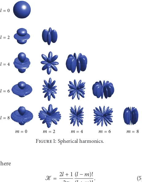
The order𝑙specifies the number of polynomial terms that a harmonic function contains. Relatively smooth functions can be obtained using low order spherical harmonics, with increasing order corresponding to an increased number of frequencies captured by the spherical harmonics. The higher the order, the more precise the approximation. Figure 1 shows the spherical harmonics for even orders up to𝑙 = 8—note that 𝑌−𝑚
𝑙 is the reflection of𝑌𝑙𝑚.
The expression of spherical harmonics uses complex domain functionals in (2). However, for ease of program-ming, and since many of the desired properties are still present, only the real part of𝑌𝑙𝑚is used, denoted by𝑌𝑅𝑚𝑙 . This is calculated as follows:
𝑌𝑅𝑚𝑙 (𝜃, 𝜙)
={{ {
K1/2𝑃𝑚
𝑙 (cos𝜃)sin(𝑚𝜙) if 𝑚 ≥ 0
(−1)−𝑚K1/2𝑃𝑚
𝑙 (cos𝜃)cos(−𝑚𝜙) otherwise,
m = 8 m = 6
m = 4 m = 2
[image:3.600.57.288.73.368.2]m = 0 l = 8 l = 6 l = 4 l = 2 l = 0
Figure 1: Spherical harmonics.
where
K= 2𝑙 + 1 2𝜋
(𝑙 − 𝑚)!
(𝑙 + 𝑚)!. (5)
The function in (1) may be solved for 𝑎𝑙𝑚 to calculate the weighting of each basis function and thereby allow an analytical representation of the surface, using the inverse transform known as the spherical harmonics transform:
𝑎𝑚 𝑙 = ∫
2𝜋
0 ∫
𝜋
0 𝑓 (𝜃, 𝜙) 𝑌 𝑚∗
𝑙 (𝜃, 𝜙)sin𝜃d𝜃d𝜙. (6)
However, this is often not possible to solve. As an alternative, (1) can be written as a series of linear equations in matrix form, for some finite𝑙maxon some discrete sampling of the surface,𝑓𝑖= 𝑓(𝜃𝑖, 𝜙𝑖), for1 ≤ 𝑖 ≤ 𝑛. The system is then solved for coefficients𝑎𝑚𝑙 ,∀𝑚, 𝑙:
(
𝑦1,1 𝑦1,2 ⋅ ⋅ ⋅ 𝑦1,𝑘 𝑦2,1 𝑦2,2 ⋅ ⋅ ⋅ 𝑦2,𝑘 ... ... d ...
𝑦𝑛,1 𝑦𝑛,2 ⋅ ⋅ ⋅ 𝑦𝑛,𝑘 ) (
𝑎1 𝑎2 ... 𝑎𝑘
) = ( 𝑓1 𝑓2 ... 𝑓𝑛
) , (7)
where𝑦𝑖,𝑗= 𝑌𝑅𝑚𝑙 (𝜃𝑖, 𝜙𝑖),𝑗 = 𝑙2+ 𝑙 + 𝑚 + 1, and𝑘 = (𝑙max+ 1)2. The unique indexing𝑗for each pair(𝑙, 𝑚)is as used in [13].
2.2. Regularisation. The spherical harmonics basis is used to
approximate the surface using least squares optimisation. The procedure minimises the sum of the squared residuals to the curve determined by the best fit. This involves solving a set of linear equations, where, for an overdetermined system of equations,Ax=b, with x unknown, the best approximation, ̂
x is calculated such that the sum of square differences
betweenÂx and b is minimised. Often, the solution does
not exist, and instead the best approximation ofx is found, minimising the function‖Âx−b‖. This can be done more simply by solving the equivalent system of equationsA𝑇Ax=
A𝑇b. For the spherical harmonics system, in (7), the system
to approximate the weighting coefficientsx= 𝑎𝑙𝑚.
Regularisation is often used to optimise solutions. This is done by introducing additional information, usually in the form of a penalty for complexity, for example, restrictions to ensure smoothness. Tikhonov regularisation is one of the most commonly used methods for regularisation [24, 25]. The additional information introduced is described as the Tikhonov matrix, which is added to the original minimisation term, acting as a smoothness constraint. The Tikhonov matrix,Γ, can be constructed in a number of ways. One such way is to use unimodal regularisation (Γ =I) [26].
Alternatively, the construction may be based on the Laplace-Beltrami smoothing operator [27–29].
Due to the linear least squares allowing outlying points to have a disproportionate effect on the fitting, there is often a degree of noise that presents itself when fitting the spherical harmonics to the surface using higher orders of 𝑙. The noise is amplified as the order increases, due to the massive increase in the number of calculations performed. As the matrix system gets bigger, a higher number of numerical inaccuracies occur, increasing the number of outlying points generated. Consequently, constructing the Tikhonov matrix based on the Laplace-Beltrami operator is the natural choice in this case, as the regularisation introduced will smooth the harmonic signal produced. The regularisation term is introduced in minimisation term as the following constraint:
‖Ax−b‖2+]‖Γ‖2, (8)
where A is the basis matrix, x is the radii vector, b is the coefficient vector,] is a tuning parameter used to balance the fidelity of the data and the smoothness requirement [30], andΓis the Tikhonov matrix. Minimising this newly formed functional results in an equivalent solution to the following equation:
(A𝑇A+]R)x=A𝑇b, (9)
whereR= Γ𝑇Γand has the following structure:
R= (
𝑙𝑗2(𝑙𝑗2+ 1)2
d
𝑙2
max(𝑙2max+ 1) 2
) , (10)
where𝑙𝑗is the spherical harmonics order associated with the 𝑗th coefficient.
(a) (b)
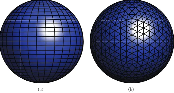
Figure 2: Example of regularly sampled meshes on sphere: UV sphere (left) and geodesic icosphere (right).
penalty would result in sparse outputs. Therefore, L2-norm penalty has been used instead of L1-norm. The multiplicity of eigenfunctions is beyond the scope of this paper and readers are invited to read [31].
2.3. Spherical Meshing. Typically surface representations as
polygonal meshes are described in Cartesian coordinates (𝑥, 𝑦, 𝑧). For the surface mesh to be represented by𝑓(𝜃, 𝜙), the mesh must be transformed into spherical polar coordi-nates (𝑟, 𝜃, 𝜙) about the origin, where𝑓(𝜃, 𝜙) = 𝑟, the distance from the origin to the point on the surface at inclination𝜃and azimuth𝜙:
𝑟 = √𝑥2+ 𝑦2+ 𝑧2
𝜃 =arccos(𝑧 𝑟)
𝜙 =arctan(𝑦 𝑥) .
(11)
On calculating the spherical harmonics coefficients and obtaining the approximation of continuous functional𝑓, a value for 𝑟 may be obtained for any given 𝜃 and 𝜙. As a result, it is possible to define a new set of points, or a new mesh, on a unit sphere (or any sphere, disregarding its radius). An example of regularly sampled spherical meshes is shown in Figure 2, which can be used to remesh an approximated surface. The mapping from polar coordinates to Cartesian coordinates is𝑥 = 𝑟sin𝜃cos𝜙,𝑦 = 𝑟sin𝜃sin𝜙, and𝑧 = 𝑟cos𝜃.
3. Implementation
3.1. Surface Parametrisation. Given a mesh, with vertices
transformed into spherical coordinates treating the geometric centre of all mesh points as the origin, a set of basis functions for angles 𝜃 and 𝜙 is calculated up to the specified order 𝑙max. Each basis function is calculated according to (4) and the values indexed in𝑛-by-𝑘matrix, where𝑛is the number of vertices in the mesh and𝑘 = (𝑙max + 1)2. As described
previously, for the𝑖th vertex, the calculated values for each basis function 𝑌𝑅𝑚𝑙 (𝜃𝑖, 𝜙𝑖) are added to the matrix at 𝑦𝑖𝑗, where𝑗 = 𝑙2+ 𝑙 + 𝑚 + 1.
The system of equations is set up as in (7), where𝑓𝑖 = 𝑟𝑖, the spherical radius value at angle(𝜃𝑖, 𝜙𝑖), and solved using the Laplace-Beltrami Tikhonov regularisation described in Section 2.2, using ]to control the added smoothness con-straint. The resulting vector of coefficients can then be used to weight spherical harmonics in the functional𝑓(𝜃, 𝜙)(1), describing the surface which the mesh represents. As the spherical harmonics series has been truncated to a maxi-mum order,𝑙max, the computed values of𝑓(corresponding to radius values 𝑟 in a spherical representation) are only approximations of the original values.
Multiplying the calculated coefficients𝑎𝑚𝑙 by the spherical harmonics values for the original set of mesh vertex angles, the residual error for each vertex can be obtained in the form
Ax−b, where A are the bases, x is the set of approximated
coefficients, andb is values of𝑓for each pair of𝜃𝑖and𝜙𝑖. The newly reapproximated vertices can also be visualised by converting the values from spherical to Cartesian coordi-nates and retaining the face information of the original mesh. This face information is in the form of a list. This list does not contain the vertex values themselves but the indices for each vertex. Therefore, each line in the list contains three (for a triangular mesh) indices that comprise a single face. The face information remains valid as long as the order of initial vertices and their approximations stay the same.
3.2. Remeshing. Once the coefficients for the mesh have been
1
0.5
0
−0.5
−1 −0.5
0 0
0.5 −1
1
(a)
0
0.8
0.6
0.4
0.2
−0.2
−0.4
−0.6
0 0
−0.5 −0.5 0.5
0.5
[image:5.600.143.459.71.289.2](b)
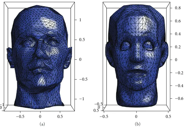
Figure 3: Two triangular meshes of human heads:Mannequin(left) andObrubovka(right).
approximation𝑓𝑟, can be converted into a set of Cartesian coordinates(𝑥𝑟, 𝑦𝑟, 𝑧𝑟)describing the remeshed surface of the original mesh. Again, face information defined on the sphere can be applied to these new vertices.
4. Results
4.1. Parametrisation. It is important for a remeshing
algo-rithm to approximate an input surface well. Therefore, there is a need to measure how close the reconstructed surface is to the original. The numerical measures used in [13] to describe the fit are the mean residual and the maximum residual, and consequently these measures are used here. The residual is calculated for each vertex in the original and approximate mesh, as described in Section 3.1, and for two given meshes, the surfaces are approximated and results given. These meshes, both representing a human head, exhibit different levels of features. They are distinguished in this paper as Mannequin and Obrubovka and shown in Figure 3. The residuals of parametrisation of the meshes by spheri-cal harmonics, solved only by linear least squares for different values of𝑙max, are given in Table 1, with reconstructed meshes shown in Figure 4. As the order of the spherical harmonics increases, the residual errors decrease. This is as expected, since a higher order captures higher frequencies in the surface and is a better representation of the structure.
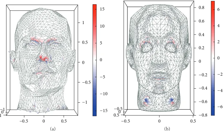
[image:5.600.309.549.370.486.2]In addition to the quantitative metrics, the resulting meshes are plotted and shaded with the local vertex residuals, shown in Figure 5. Visual analysis shows the performance of spherical harmonics as a parametrisation technique is suitable for a large proportion of a mesh, with the highest errors occurring where the curvature in the mesh is sharpest, notably the nose and brow region. As the maximum order is increased, these effects are reduced, as demonstrated by the results presented in Table 1. The results here agree with the observation that spherical harmonics perform well
Table 1: Mean (msd) and maximum (xsd) residuals for different orders of spherical harmonics parametrisation of two meshes, solved using linear least squares.
Mesh Vertices Faces 𝑙max msd xsd
Mannequin 1693 3382
10 3.526 23.093 20 2.380 19.526 40 1.341 21.384 60 0.511 16.531
Obrubovka 3301 6598
10 2.743 14.209 20 1.285 13.634 40 0.533 9.888 60 0.202 7.061
as a parametrisation technique [13]. The reconstruction in Figure 4 is visually very similar to the original mesh and spherical harmonics representation can capture main surface features from the original mesh well. However, at lower orders, very sharp features are difficult to reconstruct, as can be seen in the ears of the Mannequin mesh at𝑙max = 20.
4.2. Remeshing. Each of the meshes parametrised has been
1
0.5
0
−0.5
−1 −0.5
0 0.5
−1 1
1
0.5
0
−0.5
−1 −0.5
0 0.5
−1 1
1
0.5
0
−0.5
−1 −0.5
0 0.5
−1 1
1
0.5
0
−0.5
−1 −0.5
0 0.5
−1 1
lmax= 10 lmax= 20 lmax= 40 lmax= 60
(a)
lmax= 10 lmax= 20 lmax= 40 lmax= 60
0.8
0.6 0.4 0.2 0 −0.2 −0.4 −0.6 −0.8
0.8
0.6 0.4 0.2 0 −0.2 −0.4 −0.6 −0.8
−0.4 −0.2 0 0.2 0.4 0
−0.5
−0.5
0.5 −0.50.5
0.5
0.8
0.6 0.4 0.2
0 0
−0.2 −0.4 −0.6 −0.8 0
−0.5 −0.5
0.5
0.5
0.8
0.6 0.4 0.2
−0.2 −0.4 −0.6 −0.8 0
−0.5 −0.5
0.5
0.5
[image:6.600.60.540.72.433.2](b)
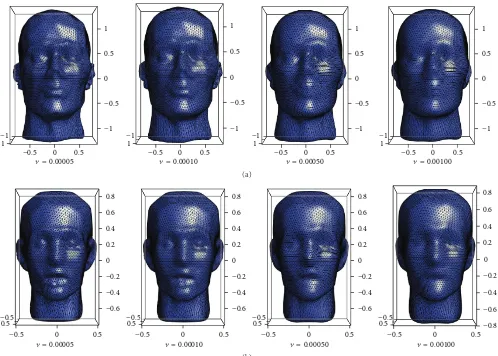
Figure 4: Original surface meshes,Mannequin(top) andObrubovka, approximated by spherical harmonics and meshed using the original vertex angles and face information using increasing values of𝑙max.
1
0.5
0
−0.5
−1
−0.5 0 0.5
−10 1
15
10
5
0
−5
−10
−15
(a)
−0.5 0 0.5
−0.50 0.5
6
4
2
0
−2
−4
−6 0.8
0.6
0.4
0.2
0
−0.2
−0.4
−0.6
−0.8
(b)
[image:6.600.114.486.485.703.2](a) (b)
(c) (f)
(d) (e)
1
0.5
0
−0.5
−1 −0.5
0 0.5
−1 1
−1
1
0.5
0
−0.5
−1 −0.5
0 0.5
−1 1
150
100
50
0
−50
−100
−150
−200 −100 0 100 200 300
0
0.8
0.6 0.4 0.2
−0.2 −0.4 −0.6 −0.8 0
0.8
0.6 0.4 0.2
−0.2 −0.4 −0.6 −0.8
0 −0.5
−0.5 0.5 −0.5
0.5
0.5
−0.4−0.2 0 0.2 0.4
1.5
1
0.5
0
−0.5
−1 −0.5 0 0.5 1
0 1
[image:7.600.60.539.68.406.2]0 50 150
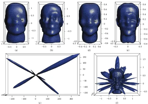
Figure 6: Surfaces represented by spherical harmonics, solved using linear least squares, remeshed with an icosphere for values of𝑙max= 10, 20, and 40 forMannequin(a–c) andObrubovka(d–f).
basis functions that would need to be calculated and utilised in the linear system.
Figure 6 shows the remeshing results for the two models. These show outlying regions affected by high frequency harmonics, which increase in noise as the order increases. At high levels, the original mesh’s structure is virtually unrecognisable in the remeshed figure. The “spikes” are amplified particularly in regions of low detail or resolution in the original mesh. The mesh created through the remeshing process inherits many properties of the given spherical sampling mesh, in this case a pseudouniform triangular grid over the entire surface. Increasing the resolution of the mesh much greater than that of the initial mesh can significantly reduce the interpolating effects of the remeshing process.
4.3. Tikhonov Regularisation. Tikhonov regularisation was
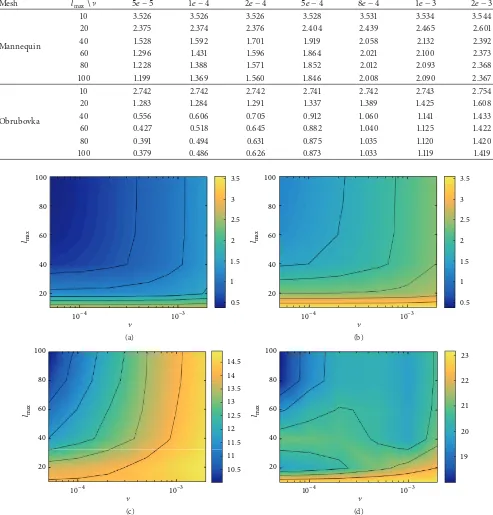
introduced to aid solving the discrete spherical harmonics transform, adding a smoothing constraint to the resulting surface representation and reducing computational runtime in solving the linear system [32]. Residuals errors of the results for the original meshes parametrised using Tikhonov regularisation are shown in Table 2 for increased order,𝑙max, and various values of ], the weighting coefficient for the Tikhonov matrix. Note that when]= 0, the result is the linear
least squares solution. The residuals for the results of varied
combinations of]and𝑙maxare shown in Figure 8, showing the lowest residuals (both mean and maximum) for high order (𝑙max) and low regularisation (]).
Using the same process for remeshing, the regularised coefficients are used to approximate the meshes on finer, more uniform sampling. The effects of the smoothing reduce the impact of the high frequency harmonics, allowing high orders to increase refinement of the mesh, while avoiding numerical errors and “spiky” outliers. The resulting meshes using the icosphere sampling are shown in Figure 7 at different orders, showing the effectiveness of the remeshing technique and the substantial improvement regularisation brings about compared to the results using only linear least squares (Figure 6).
1
0.5
0
−0.5
−1 −0.5
0 0.5
−1 1
1
0.5
0
−0.5
−1 −0.5
0 0.5
−1 1
1
0.5
0
−0.5
−1 −0.5
0 0.5
−1 1
1
0.5
0
−0.5
−1 −0.5
0 0.5
−1 1
= 0.00005 = 0.00010 = 0.00050 = 0.00100
(a)
0
0.8
0.6 0.4 0.2
−0.2 −0.4 −0.6
0 −0.5
−0.50.5
0.5
0
0.8
0.6 0.4 0.2
−0.2 −0.4 −0.6
0 −0.5
−0.50.5
0.5
0
0.8
0.6 0.4 0.2
−0.2 −0.4 −0.6
0 −0.5
−0.50.5
0.5
0
0.8
0.6 0.4 0.2
−0.2 −0.4 −0.6 −0.8 0
−0.5 −0.50.5
0.5
= 0.00005 = 0.00010 = 0.00050 = 0.00100
[image:8.600.51.549.69.425.2](b)
Figure 7: Remeshed (using an icosphere) surfaces forMannequin(top) andObrubovkaapproximated by regularised spherical harmonics
(𝑙max= 100) for increased values of regularisation coefficient].
combination of high order 𝑙max = 100 and very low regularisation coefficient,] = 5𝑒 − 5, gives global minima
in the residual plots for the combinations tested. Visually, the remeshed plots show clearly retained structure over the regular grid (Figure 7) without the presence of the “spikes” seen in the nonregularised linear least squares representation.
4.4. Surface Inpainting. When surface meshes are created,
they may contain undersampled regions rendering the mesh incomplete with holes. For example, when using 3D range scanners to produce a mesh of an object, there may be holes on the surface of the mesh due to occlusion. In order to use the mesh for processes such as animation, texturing, and simulation, the holes on the surface need to be closed in a preprocessing step. Filling these holes is known as surface inpainting. Current methods for surface inpainting incorporate hole detection schemes that use the local context of the surface on the boundary of the hole in order to make a judgement on how to close the hole. Information gathered by the local context includes the surface curvature and sampling rate. Locating the hole on a mesh, especially a large highly sampled mesh, can be computationally expensive.
Table 2: Mean (msd) residuals for different orders of spherical harmonics parametrisation of two meshes, solved using increasing degrees of Tikhonov regularisation.
Mesh 𝑙max\] 5𝑒 − 5 1𝑒 − 4 2𝑒 − 4 5𝑒 − 4 8𝑒 − 4 1𝑒 − 3 2𝑒 − 3
Mannequin
10 3.526 3.526 3.526 3.528 3.531 3.534 3.544
20 2.375 2.374 2.376 2.404 2.439 2.465 2.601
40 1.528 1.592 1.701 1.919 2.058 2.132 2.392
60 1.296 1.431 1.596 1.864 2.021 2.100 2.373
80 1.228 1.388 1.571 1.852 2.012 2.093 2.368
100 1.199 1.369 1.560 1.846 2.008 2.090 2.367
Obrubovka
10 2.742 2.742 2.742 2.741 2.742 2.743 2.754
20 1.283 1.284 1.291 1.337 1.389 1.425 1.608
40 0.556 0.606 0.705 0.912 1.060 1.141 1.433
60 0.427 0.518 0.645 0.882 1.040 1.125 1.422
80 0.391 0.494 0.631 0.875 1.035 1.120 1.420
100 0.379 0.486 0.626 0.873 1.033 1.119 1.419
100
80
60
40
20
3.5
3
2.5
2
1.5
1
0.5 lmax
10−4 10−3
(a)
3.5
3
2.5
2
1.5
1
0.5 100
80
60
40
20 lmax
10−4 10−3
(b)
14.5 14 13.5 13 12.5 12 11.5 11 10.5 100
80
60
40
20 lmax
10−4 10−3
(c)
23
22
21
20
19 100
80
60
40
20 lmax
10−4 10−3
(d)
Figure 8: Error plots showing the mean (top row) and max residual error for regularised spherical harmonics reconstruction ofObrubovka (left column) andMannequin, showing values for]against𝑙max. Note that]values are plotted on a log scale.
5. Conclusions
This paper proposes a technique for remeshing using spher-ical harmonics as a parametrisation technique. By repre-senting a mesh through a finite series of spherical basis functions with increasing frequencies, it has been possible
cal harmonics allows for the resolution of the model to be altered with ease. This method could be used as a preprocessing algorithm for processes that require a reg-ular mesh such as animation, texturing, simulation, and modelling.
The approach presented was tested with both quantitative and visual analysis of results. Spherical harmonics perform well as a parametrisation technique, although when the basis equations were solved using only linear least squares a source of error occurred in regions with little detail available in the original mesh. This was observed in the remeshing, with errors increasing with basis order, a result of using higher frequencies to represent the surface. As a result, Tikhonov regularisation as a smoothing measure was investigated and found to be effective at constraining high frequency errors without significantly reducing the approximated detail. The Tikhonov matrix used is based on the Laplace-Beltrami smoothing operator, so for highly weighted regularisation, oversmoothing may occur. The best results were observed with high spherical harmonics order and low (nonzero) levels of regularisation.
The computational complexity of this method is affected by two main variables: the number of vertices, 𝑛, of the original mesh to be remeshed and the value of𝑙max. The larger the values of𝑛and𝑙max, the more the basis functions that need to be computed. With more basis functions, there are more computations required in solving the linear system in (9). The complexity of calculating the basis functions becomes 𝑂(𝑛𝑙max2).
The technique has some limitations. The first is a limita-tion regarding features in the original mesh. It is common for vertices to be placed along edges of a surface in order to capture sharpness of the edge. However, remeshing may not account for these features, and the surfaces are by nature rounded by spherical harmonics. Research efforts in the future may be focussed towards feature detection and feature preservation schemes, for example, searching for sharp edges in the mesh and preserving these dur-ing the remeshdur-ing by placdur-ing vertices along the original edges.
Additionally, there is compromise between regularisation parameter and spherical harmonics order, which are inversely proportional in producing the highest accuracy. Despite this, if the weight of the regularisation matrix in solving the spherical harmonics system is too low, the noisy spikes can occur during remeshing. This can be manually selected, or similar effects may be investigated with regularisation in alternative solvers, such as those discussed in [13], which deals with calculating approximations of high resolution meshes.
In its present form, the technique here does not explicitly deal with the presence of occluded regions in its mapping to spherical domain. This is especially important in higher genus surfaces or those with structural complexities, such as the ears of the Stanford bunny. Ongoing research is investigating surface segmentation to remesh individual components. The main challenge here is combining remeshed components in a seamless way.
The authors declare that there is no conflict of interests regarding the publication of this paper.
References
[1] H. Borouchaki, P. Laug, and P.-L. George, “Parametric surface meshing using a combined advancing-front generalized delau-nay approach,”International Journal for Numerical Methods in Engineering, vol. 49, no. 1-2, pp. 233–259, 2000.
[2] Y. Zheng, N. P. Weatherill, and O. Hassan, “Topology abstrac-tion of surface models for three-dimensional grid generaabstrac-tion,” Engineering with Computers, vol. 17, no. 1, pp. 28–38, 2001. [3] D. L. Marcum, “Efficient generation of high-quality
unstruc-tured surface and volume grids,”Engineering with Computers, vol. 17, no. 3, pp. 211–233, 2001.
[4] P. Laug and H. Borouchaki, “Interpolating and meshing 3D surface grids,”International Journal for Numerical Methods in Engineering, vol. 58, no. 2, pp. 209–225, 2003.
[5] B. L´evy, S. Petitjean, N. Ray, and J. Maillot, “Least squares conformal maps for automatic texture atlas generation,”ACM Transactions on Graphics, vol. 21, no. 3, pp. 362–371, 2002. [6] Y. Ito and K. Nakahashi, “Direct surface triangulation using
stereolithography data,”AIAA Journal, vol. 40, no. 3, pp. 490– 496, 2002.
[7] E. B´echet, J.-C. Cuilliere, and F. Trochu, “Generation of a finite element MESH from stereolithography (STL) files,” Computer-Aided Design, vol. 34, no. 1, pp. 1–17, 2002.
[8] D. Wang, O. Hassan, K. Morgan, and N. Weatherill, “Enhanced remeshing from STL files with applications to surface grid gen-eration,”Communications in Numerical Methods in Engineering, vol. 23, no. 3, pp. 227–239, 2007.
[9] E. Marchandise, G. Comp`ere, M. Willemet, G. Bricteux, C. Geuzaine, and J.-F. Remacle, “Quality meshing based on STL triangulations for biomedical simulations,”International Jour-nal for Numerical Methods in Biomedical Engineering, vol. 26, no. 7, pp. 876–889, 2010.
[10] D. M. B. de Siqueira, M. O. Freitas, J. B. Cavalcante-Neto, C. A. Vidal, and R. J. da Silva, “An adaptive parametric surface mesh generation method guided by curvatures,” inProceedings of the 22nd International Meshing Roundtable, pp. 425–443, Springer, 2014.
[11] U. Labsik, K. Hormann, and G. Greiner, “Using most isometric parameterizations for remeshing polygonal surfaces,” in Pro-ceedings of the Theory and Applications Geometric Modeling and Processing, pp. 220–228, IEEE, Hong Kong, China, April 2000. [12] P. Alliez, G. Ucelli, C. Gotsman, and M. Attene, “Recent
advances in remeshing of surfaces,” in Shape Analysis and Structuring, pp. 53–82, Springer, Berlin, Germany, 2008. [13] L. Shen and M. K. Chung, “Large-scale modeling of parametric
surfaces using spherical harmonics,” inProceedings of the 3rd International Symposium on 3D Data Processing, Visualization, and Transmission (3DPVT ’06), pp. 294–301, IEEE, Chapel Hill, NC, USA, June 2006.
[14] J.-F. Remacle, C. Geuzaine, G. Comp`ere, and E. Marchandise, “High-quality surface remeshing using harmonic maps,” Inter-national Journal for Numerical Methods in Engineering, vol. 83, no. 4, pp. 403–425, 2010.
Conference and Exhibition on Computer Graphics and Interactive Techniques (SIGGRAPH ’07), ACM, San Diego, Calif, USA, August 2007.
[16] E. Praun and H. Hoppe, “Spherical parametrization and rem-eshing,”ACM Transactions on Graphics, vol. 22, no. 3, pp. 340– 349, 2003.
[17] P. Liu, Y. Wang, D. Huang, Z. Zhang, and L. Chen, “Learning the spherical harmonic features for 3-D face recognition,”IEEE Transactions on Image Processing, vol. 22, no. 3, pp. 914–925, 2013.
[18] R. Green, “Spherical harmonic lighting: the gritty details,” in Proceedings of the Archives of the Game Developers Conference (GDC ’03), vol. 56, 2003.
[19] J. Feinauer, A. Spettl, I. Manke et al., “Structural characteriza-tion of particle systems using spherical harmonics,”Materials Characterization, vol. 106, pp. 123–133, 2015.
[20] S. N. Sotiropoulos, L. Bai, P. S. Morgan, C. S. Constantinescu, and C. R. Tench, “Brain tractography using Q-ball imaging and graph theory: improved connectivities through fibre crossings via a model-based approach,”NeuroImage, vol. 49, no. 3, pp. 2444–2456, 2010.
[21] S. N. Sotiropoulos, L. Bai, and C. R. Tench, “Fuzzy anatomical connectedness of the brain using single and multiple fibre ori-entations estimated from diffusion MRI,”Computerized Medical Imaging and Graphics, vol. 34, no. 6, pp. 504–513, 2010. [22] S. N. Sotiropoulos, L. Bai, P. S. Morgan, D. Auer, C. S.
Constantinescu, and C. R. Tench, “A regularized two-tensor model fit to low angular resolution diffusion images using basis directions,”Computerized Medical Imaging and Graphics, vol. 34, no. 6, pp. 504–513, 2010.
[23] E. J. Garboczi, “Three-dimensional mathematical analysis of particle shape using X-ray tomography and spherical harmon-ics: application to aggregates used in concrete,”Cement and Concrete Research, vol. 32, no. 10, pp. 1621–1638, 2002.
[24] T. Poggio, H. Voorhees, and A. Yuille, “A regularized solution to edge detection,”Journal of Complexity, vol. 4, no. 2, pp. 106–123, 1988.
[25] P. C. Hansen, “Regularization tools: a matlab package for analysis and solution of discrete ill-posed problems,”Numerical Algorithms, vol. 6, no. 1-2, pp. 1–35, 1994.
[26] C. P. Hess, P. Mukherjee, E. T. Han, D. Xu, and D. B. Vigneron, “Q-ball reconstruction of multimodal fiber orientations using the spherical harmonic basis,”Magnetic Resonance in Medicine, vol. 56, no. 1, pp. 104–117, 2006.
[27] B. Neuman, C. Tench, and L. Bai, “Laplace-Beltrami regu-larization for diffusion weighted imaging,” inProceedings of the Annual Conference in Medical Image Understanding and Analysis (MIUA ’12), 2012.
[28] B. P. Neuman, C. Tench, and L. Bai, “Direct reconstruction of fibre orientation using discrete ground truth interpolation,” in Proceedings of the 9th IEEE International Symposium on Biomedical Imaging: From Nano to Macro (ISBI ’12), pp. 18–21, Barcelona, Spain, May 2012.
[29] B. Neuman, C. Tench, and L. Bai, “Reliably estimating the diffusion orientation distribution function from high angular resolution diffusion imaging data,” inProceedings of the Medical Image Understanding and Analysis Conference (MIUA ’11), pp. 23–28, 2011.
[30] D. Casta˜no and A. Kunoth, “Multilevel regularization of wavelet based fitting of scattered data—some experiments,”Numerical Algorithms, vol. 39, no. 1–3, pp. 81–96, 2005.
[31] M. K. Chung, Computational Neuroanatomy: The Methods, 2013.
Submit your manuscripts at
http://www.hindawi.com
Hindawi Publishing Corporation
http://www.hindawi.com Volume 2014
Mathematics
Journal ofHindawi Publishing Corporation
http://www.hindawi.com Volume 2014 Mathematical Problems in Engineering
Hindawi Publishing Corporation http://www.hindawi.com
Differential Equations International Journal of
Volume 2014
Hindawi Publishing Corporation
http://www.hindawi.com Volume 2014
Mathematical PhysicsAdvances in
Complex Analysis
Journal ofHindawi Publishing Corporation
http://www.hindawi.com Volume 2014
Optimization
Journal ofHindawi Publishing Corporation
http://www.hindawi.com Volume 2014
Combinatorics
Hindawi Publishing Corporation
http://www.hindawi.com Volume 2014 International Journal of
Journal of
Hindawi Publishing Corporation
http://www.hindawi.com Volume 2014
Function Spaces
Abstract and Applied Analysis
Hindawi Publishing Corporation
http://www.hindawi.com Volume 2014
International Journal of Mathematics and Mathematical Sciences
Hindawi Publishing Corporation http://www.hindawi.com Volume 2014
The Scientific
World Journal
Hindawi Publishing Corporationhttp://www.hindawi.com Volume 2014
Discrete Dynamics in Nature and Society
Hindawi Publishing Corporation
http://www.hindawi.com Volume 2014
Discrete Mathematics
Journal ofHindawi Publishing Corporation
http://www.hindawi.com Volume 2014 Hindawi Publishing Corporationhttp://www.hindawi.com Volume 2014