Demagnetisation analysis for Halbach array configurations in electrical machines



Abstract — This paper proposes and investigates an analytical method for assessing the risk of potential, irreversible demagnetisation in the PMs of electrical machines, equipped with n-stages, Halbach arrays. The higher risk of demagnetisation, synonymous with Halbach arrays imposes that the method be both load and temperature dependant. In fact, the proposed method studies the magnetic field distribution in the air-gap and PM region, for various operating temperatures and expresses these fields as analytical expressions for the no-load and peak load conditions. The model can cater for Halbach arrays with up to n stages, thus making it a versatile tool that can be utilised for various Halbach configurations. Finite element analysis is used to validate the method.

The analytical tool is then used for the design and analysis of a high torque density, outer rotor, traction motor. The motor is for an aerospace application and its operating duty cycle imposes very high, short time, peak load conditions at elevated temperatures, posing an elevated risk of irreversible, PM demagnetisation. The model is used to investigate various Halbach configurations for this application, in order to reduce the demagnetisation risk and also improve the general performance of the machine. The analytical method thus provides a computationally efficient tool that can be used to predict and prevent demagnetisation in Halbach-equipped, electrical machines operating in harsh environments such as the aerospace sector.

Index Terms — aerospace, demagnetisation, Halbach arrays, torque density, permanent magnets

I. INTRODUCTION

LECTRICAL machines for mobile applications such as the rail, automotive and aerospace industries are usually constrained with strong requirements of power and torque density. On top of this, reliability, efficiency and availability are also additional requirements.

From all the range of electrical machines available today, it is generally known that permanent magnet (PM) machines are able to achieve excellent torque and torque density performances, very high efficiencies and low losses [1]. Their torque/force density capabilities [2, 3] and the fault tolerance performances [4, 5] are well documented. However apart from

Manuscript submitted XX, 2014.

This work was partly supported by the “EU FP7 funding via the Clean Sky JTI – Systems for Green Operations ITD”.

Michael Galea ([email protected], phone: 0044-115-748-4961), Luca Papini ([email protected]), He Zhang ([email protected]), Tahar Hamiti ([email protected]) and Chris Gerada ([email protected]) are with the Power Electronics, Machines and Control (PEMC) group in the Faculty of Engineering of the University of Nottingham, Nottingham, NG7 2RD, UK.

the economic burden related to magnet material, other disadvantages concerning such machines are the always present no-load flux, the natural intolerance towards high temperatures [6] and the risk of irreversible demagnetisation.

An interesting but highly challenging variation of the conventional surface mount PM (SMPM) and internal PM (IPM) configurations is the use of Halbach arrays [7]. The air-gap flux density and the torque capability of a PM machine can benefit greatly from the use of such arrays. Various works [8, 9] document how adopting such a configuration enhances the sinusoidal shape of the air-gap flux density Bg, thus

improving the ratio of the fundamental air-gap flux density component Bg1 to the total Bg. A high value of this ratio

ameliorates the torque capability of the machine [8], as it is

Bg1 that actually produces the torque, whilst Bg has other

effects such as on the saturation levels of the machine. As mentioned above, one of the main requirements for mobile applications is the high torque density capability of the machines [10]. Due to this, there is an increasing interest in applying Halbach arrays for machines working in harsh environments. The improvements for machines equipped with Halbach arrays are documented in several comparative studies [7, 11]. These arrays present a number of issues that must be taken into account, with the major problem being the higher risk of demagnetisation [8]. In a Halbach array, each complete pole is assembled out of a number of segments or stages nstg

that are magnetised in different directions. The proximity of a segment to another intrinsically creates reverse magnetic fields that can demagnetise parts (usually the corners) of the segment next to it, even at no load. The demagnetisation risk is in general lower for a higher nstg [12], however smaller nstg arrays

(such as quasi-Halbach) are popular because of the reduction in costs, manufacturing and assembly procedures when compared to arrays with a higher number of stages.

Apart from all this, operation in harsh environments can also mean operating with very high temperatures and with extremely high electric loading Arms, all factors contributing to

an increase in potential PM demagnetisation. In order to enhance the reliability figures of such machines, then extensive demagnetisation analyses must be applied to the machine under the worst case operating conditions, i.e. at the maximum operating temperature Tmax and the maximum Arms

for the peak load condition. Such analyses help the machine designer achieve a comprehensive understanding of the behaviour of the PMs of the machine and thus design the machine with the minimum PM material required for the known operating conditions.

M. Galea, L. Papini, H. Zhang, C. Gerada and T. Hamiti

Demagnetisation Analysis for Halbach Array

Configurations in Electrical Machines

A relatively easy, but computationally inefficient method to do this comprises the use of time-dependant, finite element (FE) analysis. However, this can be highly time-consuming as for every time step considered, the PMs need to be evaluated in their entirety and requiring very fine meshing. At this point it is also worth mentioning that a higher nstg would require

even finer meshing, resulting in even longer solution times This paper thus proposes an analytical technique that investigates the potential of partial demagnetisation in Halbach-equipped, PM machines. The proposed model first establishes the magnetic field distribution due to the PMs on no load and then the field distribution due to the stator armature. By considering these fields in the spatial location of the PMs, the model is able to analyse the PMs and give an accurate prediction of any potential demagnetisation (complete or partly). For transient problems with a large number of steps, then this technique represents a considerable advantage in terms of reducing computational time. As vessel to test and investigate this technique, a high torque density, aerospace, traction motor [3, 12] is used. The machine is an outer rotor, Halbach-equipped, PM motor, capable of a peak torque tpk of 7kNm at a current density Jpk of 38A/mm2. The

technique is validated by FE analysis. It is shown how due to the challenging operating conditions, the motor is extremely prone to irreversible demagnetisation, and thus the technique is used to investigate alternative Halbach configurations in order to minimise the demagnetisation effects.

II. ANALYTICAL MODELLING OF MAGNETIC FIELD

DISTRIBUTIONS

A simplified analytical model can be implemented to evaluate the field distribution in the main region of the machine under investigation. The overall machine domain can be split into 3 concentric cylindrical regions, namely the air-gap region, the PMs region and the rotor region. These regions feature relative permeability and residual magnetisation according to the constitutive properties of the adopted materials. Modelling of the air-gap and the rotor region is done similar to that proposed in [13, 14].

A. General model of the PM region

The field distribution can be estimated by means of the governing equations expressed in terms of magnetic vector potential [15-17]. Eddy-current effects are neglected in the following analysis, thus for the air-gap, stator and rotor regions, the governing equation is as described by (1), where A is the magnetic vector potential.

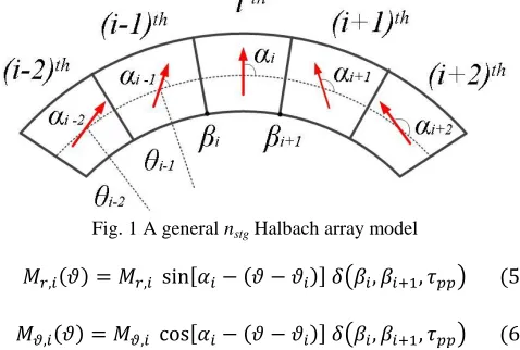
∇2_{𝑨 = 0 (1)} The PMs region can be modelled as a ring of continuous material featuring discrete magnetisation direction vectors, varying with respect to the angular position, as shown in Fig. 1. Thus, the governing equation for the PMs region is as described in (2), where μ0 is the vacuum magnetic permeability and M is the residual magnetisation vector.

∇2_{𝑨 = −𝜇}

0(∇ × 𝑴) (2) The field distribution is evaluated neglecting the end region effects, thus leading to a simplified formulation of the problem

by considering only the planar cross section orthogonal to the axial development of the device [13, 15-18]. Considering a polar coordinate reference frame, M can be decomposed in its radial Mr and tangential Mϑ components as a function of the

angular coordinate [16, 17]. Considering that an nstg Halbach

array structure consists of a number of magnet elements npm

with each element having a different magnetisation direction, then npm is described by (3), while M is as given by (4).

𝑛𝑝𝑚 = 2 𝑛𝑠𝑡𝑔− 2 (3)

𝑴(𝜗) = 𝑀𝑟(𝜗)𝑟̂ + 𝑀𝜗(𝜗)𝜗̂ = ∑ 𝑀𝑟,𝑖(𝜗)𝑟̂ + 𝑀𝜗,𝑖(𝜗)𝜗̂ 𝑛𝑠𝑡𝑔

𝑖=1

(4)

Fig. 1 illustrates a general nstg Halbach array structure. For

such a structure, if each PM segment is considered to have a constant, uniform magnetisation direction [19], then the components of M featured by the ith stage of the array can be found from (5) and (6), where ϑi is the angular position of the

magnet, αi is the angle of M with respect to the radial

direction, βi is the angular position of the left side of the ith

segment and τpp is the pair-pole pitch. The step function

δ(a,b,c) is of unitary amplitude between a and b and periodic in the interval [0 : c].

Fig. 1 A general nstg Halbach array model

𝑀𝑟,𝑖(𝜗) = 𝑀𝑟,𝑖 sin[𝛼𝑖− (𝜗 − 𝜗𝑖)] 𝛿(𝛽𝑖, 𝛽𝑖+1, 𝜏𝑝𝑝) (5)

𝑀𝜗,𝑖(𝜗) = 𝑀𝜗,𝑖 cos[𝛼𝑖− (𝜗 − 𝜗𝑖)] 𝛿(𝛽𝑖, 𝛽𝑖+1, 𝜏𝑝𝑝) (6)

Using (5) and (6), the effect of the span Tm of the PM

segments can be investigated. A perceived advantage of this model is that by appropriate modulation of Tm and/or the

magnetisation direction of each segment, then the harmonic content of Bg can be improved. A quasi-sinusoidal flux density distribution can be achieved by setting the magnetisation directions as described by (7).

𝛼𝑖= 2𝜋(𝑖 − 1)_𝑛

𝑝𝑚 (7)

B. The field distribution solution

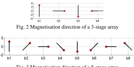
Fig. 2 Magnetisation direction of a 3-stage array

Fig. 3 Magnetisation direction of a 5-stage array

Considering the electromagnetic and geometrical features of the modelled structures, then a Fourier decomposition (with respect to ϑ) of the field quantities A and M can be done, where A is calculated as shown in (8).

𝐴𝑧(𝑟, 𝜗) = 𝑅𝑒 {∑ 𝐴̂𝑧ℎ(𝑟)𝑒−𝑗ℎ𝑝𝜗 ∞

ℎ=0

} (8)

By the superposition principle properties of the Fourier decomposition, then each single space harmonic can be taken into account separately [13]. Applying the above to the structure of Fig. 2, then its M components and their Fourier approximated function Mff are achieved as shown in Fig. 4.

The same is done for the array of Fig. 3 as shown in Fig. 5.

Fig. 4 Mr, Mϑ and respective Mff for nstg = 3

Fig. 5 Mr, Mϑ and respective Mff for nstg = 5

For the vector potential A, only the z-component (dependent only on the tangential and radial coordinates) is considered, while M is assumed to feature only the radial and tangential components (dependent only on ϑ). According to Maxwell’s equations, the field strength and the flux density can only be expressed into their radial and tangential components. Applying Fourier decomposition [13], then the field quantities (dependent on r and ϑ) can be described by the governing field equations of (9) and (10), where Â(r) is the complex value of

A for the hth space harmonic. 𝜕2

𝜕𝑟2𝐴̂(𝑟) +

1 𝑟

𝜕

𝜕𝑟𝐴̂(𝑟) − ( ℎ𝑝

𝑟)

2

𝐴̂(𝑟) = 0 (9)

𝜕2 𝜕𝑟2𝐴̂(𝑟) +

1 𝑟

𝜕

𝜕𝑟𝐴̂(𝑟) − ( ℎ𝑝

𝑟) 2

𝐴̂(𝑟) = −𝜇 𝑟[

𝜕

𝜕𝑟𝑀̂𝜗− 𝑗ℎ𝑝𝑀̂𝑟] (10)

The general solution of (9) and (10) is given in (11) and (12), where C1, C2, C3, and C4 are the integration constants,

evaluated according to a consistent system of conditions on the boundary of the domain and on the separation surfaces between regions (for regions featuring different material properties) [13, 16]. As proposed in [17], the parameter φh which is described in (13) is used to define the particular solution of (12).

𝐴̂(𝑟) = 𝐶1𝑟ℎ𝑝+ 𝐶2𝑟−ℎ𝑝 (11)

𝐴̂(𝑟) = 𝐶3𝑟ℎ𝑝+ 𝐶4𝑟−ℎ𝑝+ 𝜑ℎ𝑟 (12)

𝜑ℎ=

{

−𝜇 (𝑗ℎ𝑝𝑀̂𝑟−𝑀̂𝜗

(ℎ𝑝)2_{− 1} ) 𝑖𝑓 ℎ𝑝 > 1

−1 2(ln 𝑟 −

1

2) (𝑀̂𝑟+𝑀̂𝜗) 𝑖𝑓 ℎ𝑝 = 1

(13)

Equations (11) – (13) consider only the effects of the PMs (i.e. at no-load). In order to model the effects that the stator supply has on the PMs region, a current sheet hǨs and the

interface boundary conditions (between regions) described by (14) and (15) are defined, where B is the flux density distribution, H is the magnetic field strength distribution and n is a unitary vector normal to the interface. From (15), it can be perceived, how the model can be considered to be emulating no-load conditions when hǨs is set to 0, and on-load conditions

when hǨs is set to a finite value.

( 𝑩ℎ̂ −ℎ+1_{𝑩̂) ∙ 𝒏 = 𝟎 (14)}

( 𝑯ℎ̂ −ℎ+1𝑯̂) × 𝒏 = 𝑲ℎ̆𝑠 (15)

The current sheet is modelled into its space harmonics to take into account the slotting effect [20]. However, from (14) and (15) it can be observed how this is only valid when a finite value of hǨs is set (i.e. only for on-load conditions). In order to

of a compensating factor. This is defined in (16), where Bs is

the flux density distribution when considering slotting and 𝐵̂𝑛𝑠= 𝐵𝑠,𝑟+ 𝑗𝐵𝑠,𝜃 is the same when no slotting is considered. This last is defined as a complex number, evaluated for a non-slotted machine where the radial component of the air gap flux density 𝐵_𝑠,𝑟 is the real part and the tangential one 𝐵_𝑠,𝜃 for the complex part. As defined in [17], k is a complex constant dependent on the geometrical aspects and s=rejθ.

𝐵𝑠= 𝐵̂𝑛𝑠(

𝜕𝑘 𝜕𝑠)

∗

(16)

The resulting relations from the interface-boundary conditions (14) and (15) and the slotting effect as described in (16), evaluated for the hth space harmonic can be organized in a matrix of coefficients hD and a vector hF of known terms [13]. The matrix hD and the vector hF are related as shown in (17), where the integration constant hc can easily be found by solving this linear system.

𝑫 𝒄𝒉 _{= 𝑭}𝒉

𝒉 ₍₁₇₎

Considering the definition of the magnetic vector potential A, then the radial and tangential components of B can be defined as shown in (18) and (19) respectively. By applying the constitutive equation of materials, H can also be found.

𝐵̂𝑟(𝑟) = 𝑗

ℎ𝑝

𝑟 𝐴̂𝑧(𝑟) (18)

𝐵̂𝜗(𝑟) = −

𝜕

𝜕𝑟𝐴̂𝑧(𝑟) (19) Once each space harmonic of the field distribution is evaluated through (18) and (19), then an inverse Fourier transformation is performed, resulting in an accurate, approximated estimation of the field distribution with respect both to r and ϑ.

III. VALIDATION WITH FE ANALYSIS

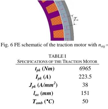
In order to validate the analytical model describing the magnetic field distribution, a FE model of the traction motor is built. Fig. 6 shows a general schematic diagram of the motor model, where the main features such as the outer rotor and the 3-stage, Halbach array can be observed. The motor, which is presented in detail in [12] is a 36 slot, 42 pole machine with an open slot configuration in order to achieve better thermal performances through the enhancement of the slot fill factor

Kfill. The machine is designed for the aerospace application

mentioned above and presented in [3, 12]. Some of the more important specifications of this model are listed in Table I, where Ipk is the peak of the current required per phase for the

peak load condition, tpk is the torque achieved during peak

load condition, lax is the axial length of the machine and Tamb

is the ambient temperature.

Fig. 6 FE schematic of the traction motor with nstg = 3,

TABLEI

SPECIFICATIONS OF THE TRACTION MOTOR tpk(Nm) 6965

Ipk (A) 223.5 Jpk (A/mm2) 38

lax (mm) 151 Tamb(°C) 50

The motor is optimised in order to achieve the highest torque density capability possible. It is beyond the scope of this paper to go into the details of the optimisation procedure, however it is important to note that special care is taken to find the optimum ratio of Tm. The PMs used for this model are

a 26/10 grade of Sm2Co17 whose demagnetisation properties [21] and curves are shown in Table II and Fig. 7, where Tpm is

the temperature of any point in the PMs.

TABLEII

PROPERTIES OF THE MAGNETIC MATERIAL Maximum Tpm(°C) 350

(BH)max (kJ/m 3

) 205

Brem (T) 1.04

Hci (kA/m) 2000

Fig. 7 Sm2Co17 demagnetisation curves

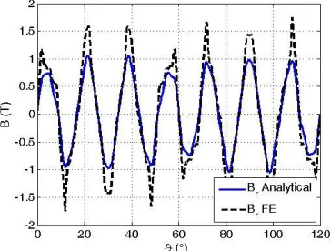
Fig. 8 and Fig. 9 compare Br and Bϑ achieved from the

Fig. 8 Br in the air-gap: FE vs. analytical

Fig. 9 Bϑ in the air-gap: FE vs. analytical

Fig. 10 Br in the PM: FE vs. analytical

Fig. 11 Bϑ in the PM: FE vs. analytical

As can be observed from Fig. 8 - Fig. 11, a very good similarity exists between the analytical and FE predicted results. Any differences can be attributed mainly to the stator slotting effects (which cannot be accurately accounted for in the analytical model) and to the inability of the analytical model to consider the same number of harmonics as the FE model (due to computational resources). However, the similarity of the results proves the adequateness of the analytical model of Section II to predict and analyse the field distributions in an electrical machine with a Halbach array.

IV. DEMAGNETISATION ANALYSIS

For a PM material such as shown in Fig. 7, irreversible demagnetisation occurs when the PM is operated below the knee point of the close loop curve (shown in red in Fig. 7). As the operating Tpm increases, this knee limit in terms of B

increases, in fact for the lower temperature curves of the Sm2Co17 material, the knee point is actually in the negative quadrant, while for a Tpm of 300°C, it is situated at

approximately 0.2T. This means that for a Tpm that is less than

250°C, demagnetisation of any point in the PM would only occur when the B at that point has been completely reversed in its direction. On the other hand, as a worst case scenario, if

Tpm is 300°C and B in any point in the direction of the PM magnetisation goes below 0.2T, then partial irreversible demagnetisation will occur at that point, resulting in an important decrease in Brem.

The demagnetisation prevention exercise is thus carried out by setting a demagnetisation proximity field Bprox as described

in (20), where Bdemag is the PM demagnetisation value (the

knee point of Fig. 7), M is a magnetisation vector indicating the direction of magnetisation and Mnorm is the norm of M.

𝐵𝑝𝑟𝑜𝑥= 𝐵𝑑𝑒𝑚𝑎𝑔− 𝐵 ∙ 𝑴 𝑀 𝑛𝑜𝑟𝑚

⁄ (20) From (20), it can be perceived that if Bprox ≤ 0, then there is

no risk of demagnetisation, while if Bprox ≥ 0, then there is a

risk of demagnetisation. It can also be observed from (20), that the more positive Bprox is, then the more important

(irreversible) the demagnetisation is. By applying the concept shown in (20) to (18) and (19), then a reliable and accurate demagnetisation prediction technique is achieved.

A. Demagnetisation on no-load

As seen above, in a Halbach array, each complete pole is assembled out of segments that are magnetised in different directions relative to each other. The proximity of a segment to another intrinsically creates reverse magnetic fields that can demagnetise parts (usually the corners) of the segment next to it, even when under no-load. In order to investigate this, the analytical models of (18) and (19) are used to create maps of

Br and Bϑ for the no-load condition and with Tpm = Tamb.

is very similar to the FE obtained result. Fig. 12 gives a potential partial demagnetisation in the axially magnetised segment of approximately 3%, while Fig. 13 shows a 2.7% demagnetisation.

Fig. 12 Analytical model (nstg = 3): no-load at Tamb

Fig. 13 FE model (nstg = 3): no-load at Tamb

The analytical models presented above are also dependant on temperature. In order to investigate and validate the analytical model’s potential to consider this important variable, then the same demagnetisation exercise on no-load is done, however this time considering a worst case operating scenario of Tpm = 300°C. The analytical model’s

demagnetisation prediction is shown in Fig. 14, whilst Fig. 15 shows the FE model’s results.

Fig. 14 Analytical model (nstg = 3): no-load at Tpm = 300°C

As can be observed from Fig. 12 and Fig. 13, a very small, negligible demagnetisation is manifested when the motor is at

Tamb, however for the worst case Tpm, it can be seen in Fig. 14

with a 23.5% potential demagnetisation and Fig. 15 (with 26.6% demagnetisation) that almost one fourth of the axially-magnetised, PM segment is partly demagnetised.

Fig. 15 FE model (nstg = 3): no-load at Tpm = 300°C

At this point, it is important to note that it is very improbable that the motor will ever be operating at 300°C, for the obvious reason that at such temperature not only the PMs would be in danger of damage but also other components such as the windings etc… However, the above (i.e. for the max Tpm

scenario) does indicate the general weakness of lower nstg

Halbach configurations in terms of demagnetisation issues.

B. Demagnetisation at peak load

The risk of demagnetisation is greatest when the machine is operating at maximum current loading. Apart from the fields due to the armature windings, the extra heat due to the copper losses can result in a general increase of the operating Tpm. An

even greater risk is experienced, if field weakening is implemented by applying finite values of the d-axis current Id,

however for this work it is assumed that the phase currents are in phase with the back-EMF.

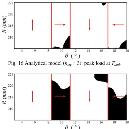
The analytical models are thus used to predict the demagnetisation of the motor for maximum Jpk. Fig. 16 shows

the analytical demagnetisation prediction for the peak load condition assuming Tamb, while Fig. 17 shows the same

assuming a worst case Tpm of 300°C. The same conditions are

then used to evaluate the demagnetisation analysis using FE analysis and the results are shown in Fig. 18a and Fig. 18b. A good similarity is again shown between the analytically predicted results and the FE obtained ones, proving the adequateness of the proposed analytical technique.

Fig. 16 Analytical model (nstg = 3): peak load at Tamb

a) Tpm = Tamb b) Tpm = 300°C

Fig. 18 FE model (nstg = 3): peak load

Apart from showcasing the reliability of the analytical technique, the results shown in the figures above, both for the no-load and the peak load condition, evidence the elevated demagnetisation risk, associated with this configuration of Halbach array. Considering the results shown in Fig. 16 and Fig. 18a for the peak load at Tamb, the potential partial

demagnetisation in the axially magnetised segment is about 16.67%. The loss for the worst case Tpm is approximately 16.67% for the radially magnetised segment and a staggering 66.67% for the axially magnetised PM. In general, it means that after the first run at peak condition, the torque performance of the machine will be drastically reduced. This situation is considered unacceptable and a solution to the problem is investigated.

V. INCREASING THE NUMBER OF STAGES

A Halbach configuration with nstg = 3, such as shown in Fig.

6, is commonly known as a quasi-Halbach array. The low nstg

implies that the angle of direction of the PM demagnetisation changes abruptly by 90° from one segment to its successive neighbour. This creates very strong fields, which can be very detrimental in terms of demagnetisation [12].

As a solution to this problem (and also to validate the analytical technique for higher nstg values), a 5-stage, Halbach

array, such as illustrated in Fig. 19 is implemented into the rotor of the traction motor. The main reasoning behind this is that with nstg = 5, the transition between the magnetisation

directions is smaller due to the increased number of stages.

Fig. 19 FE schematic of the traction motor with nstg = 5

The analytical model is used to predict the demagnetisation of the motor for both the no-load and peak load conditions assuming first Tamb and then a Tpm of 300°C. The FE model of

the motor is also tested with the same conditions. Fig. 20 and Fig. 21 show the results from the analytical model, while Fig. 22 shows the same from the FE model. For reasons of space, only the worst case scenarios of when Tpm is 300°C are shown.

Fig. 20 Analytical model (nstg = 5): no-load at Tpm = 300°C

Fig. 21 Analytical model (nstg = 5): peak load at Tpm = 300°C

a) No load b) Peak load

Fig. 22 FE model (nstg = 5): at Tpm = 300°C

As can be observed by comparing Fig. 20 to Fig. 22a and Fig. 21 to Fig. 22b, an excellent similarity between the analytical and FE results exists. For the peak load condition, the analytical model predicts a demagnetisation of 13.5% of the radially magnetised PM, while the FE model predicts 14.89%. This confirms that the analytical model behaves equally well for a higher nstg, thereby showing the versatility

of the technique in terms of the considered number of stages of the Halbach configuration.

From the application perspective, it can be observed how even with a higher nstg, the model is still susceptible to partial

demagnetisation. Fig. 22a illustrates the demagnetisation prediction of the model on no load at Tpm = 300°C. By

comparing Fig. 22a to Fig. 15, a considerable improvement in terms of demagnetisation risk can be glimpsed for these no load tests. However some demagnetisation in the top corners of the PMs is still present.

As already mentioned, it is at the peak load condition that the machine is most susceptible to partial demagnetisation. Fig. 22b shows the results obtained at peak load from the FE model with Tpm = 300°C. Comparing these results with those

shown in Fig. 18b, a considerable improvement has been achieved. However for this peak load condition for the worst case Tpm, a loss of approximately 15% of PM material is still

VI. IMPROVEMENT AND PRACTICAL SOLUTION

Having validated the worthiness of the analytical model and confirmed its reliability by adequate FE analysis, then to minimise the demagnetisation shown in Fig. 21 and Fig. 22b, an alternative design is considered. This part of the work is included only to show the final solution proposed for the application at hand and to showcase how different methods of avoiding demagnetisation can be implemented depending on the application requirements.

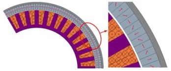
In order to achieve the required minimisation of demagnetisation area and also to reduce PM area, it is decided to physically separate the adjacent PMs by small air-gaps between each individual PM. This concept is shown in Fig. 23, where it can be observed how the space between the PMs results in the PMs having a rectangular shape. This is also an advantage in terms of manufacturing. The rectangular shape of the PMs reduces the amount of wasted material, limits manufacturing time and simplifies assembly procedures, thus scaling down the traditionally elevated costs of such a high stage number Halbach arrangement by a considerable factor.

Fig. 23 Practical solution for the traction motor

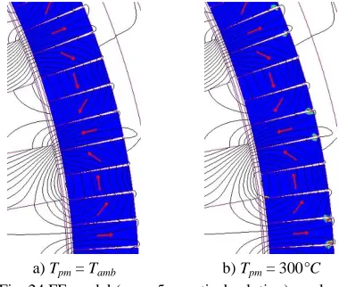
The results of the demagnetisation analysis for the proposed solution are illustrated in Fig. 24 for the no-load condition and Fig. 25 for the peak load condition. The no-load condition for worst case Tpm shown in Fig. 24b shows the small, negligible

amount of inevitable demagnetisation present in the top corners of the PMs.

a) Tpm = Tamb b) Tpm = 300°C

Fig. 24 FE model (nstg = 5, practical solution): no-load

Fig. 25 shows the effects of the fields created by the armature at the peak load condition especially at the bottom corners of the main, axially magnetised PMs. This means that if during peak load conditions, the rotor of the machine

operates at temperatures near to 300°C a small amount of material (less than 2% for each individual PM) would be partially demagnetised.

a) Tpm = Tamb b) Tpm = 300°C

Fig. 25 FE model (nstg = 5, practical solution): peak load

Even though this 2% material demagnetisation only occurs if Tpm = 300°C, in order to investigate the potential effect on

the torque performance of the machine, the demagnetised corners (shown in Fig. 25b) are removed and assigned as air. From this study, the reduction in the performance of the machine due to this 2% material degradation is minimum and can be considered negligible. This analysis is not shown here as it goes beyond the scope of this paper.

Thus, as indicated from all the above, this solution represents the best performance in terms of demagnetisation. In fact, this 5-stage Halbach array with air-gaps between the PMs reduces and virtually nullifies the irreversible, partial demagnetisation issues encountered during this work.

VII. CONCLUSION

An analytical technique for assessing partial, irreversible demagnetisation in PM machines equipped with n-stages, Halbach arrays has been proposed and investigated in this paper. The worthiness of the analytical model has been validated with representative FE models. The technique has been shown to give accurate results even when considering different variables and situations such as for different number of stages in the Halbach array and different current loading conditions ranging from no load to maximum peak load.

The vessel chosen to study the demagnetisation prediction exercise presented in this paper, was a high performance, high torque density, aerospace, traction motor. It was shown how due to the extreme conditions and highly challenging performance specifications, this particular motor is very prone to demagnetisation. Alternative solutions to this problem were proposed and investigated and a solution that minimises the demagnetisation risk was identified.

In this paper, the proposed analytical tool has been shown to be an accurate and computationally efficient tool for evaluating and predicting the irreversible, partial demagnetisation that PM motors comprising n-stages, Halbach arrays are prone to.

REFERENCES

[1] J. F. Gieras and M. Wing, Permanent Magnet Motor Technology: Design and Applications. New York, USA: Marcel Dekker Inc., 2002.

[2] C. Gerada and K. J. Bradley, "Integrated PM Machine Design for an Aircraft EMA," Industrial Electronics, IEEE Transactions on,

vol. 55, pp. 3300-3306, 2008.

[3] T. Raminosoa, T. Hamiti, M. Galea, and C. Gerada, "Feasibility and electromagnetic design of direct drive wheel actuator for green taxiing," in Energy Conversion Congress and Exposition (ECCE), 2011 IEEE, 2011, pp. 2798-2804.

[4] N. Bianchi, S. Bolognani, Pre, x, and M. D., "Strategies for the Fault-Tolerant Current Control of a Five-Phase Permanent-Magnet Motor," Industry Applications, IEEE Transactions on, vol. 43, pp. 960-970, 2007.

[5] T. Raminosoa, C. Gerada, N. Othman, and L. D. Lillo, "Rotor losses in fault-tolerant permanent magnet synchronous machines,"

Electric Power Applications, IET, vol. 5, pp. 75-88, 2011. [6] M. Galea, C. Gerada, T. Raminosoa, and P. Wheeler, "A Thermal

Improvement Technique for the Phase Windings of Electrical Machines," Industry Applications, IEEE Transactions on, vol. 48, pp. 79-87, 2012.

[7] Z. Q. Zhu and D. Howe, "Halbach permanent magnet machines and applications: a review," Electric Power Applications, IEE Proceedings -, vol. 148, pp. 299-308, 2001.

[8] M. Galea, T. Hamiti, and C. Gerada, "Torque density improvements for high performance machines," in Electric Machines & Drives Conference (IEMDC), 2013 IEEE International, 2013, pp. 1066-1073.

[9] S. Dwari and L. Parsa, "Design of Halbach-Array-Based Permanent-Magnet Motors With High Acceleration," Industrial Electronics, IEEE Transactions on, vol. 58, pp. 3768-3775, 2011. [10] A. Boglietti, A. Cavagnino, A. Tenconi, and S. Vaschetto, "The

safety critical electric machines and drives in the more electric aircraft: A survey," in Industrial Electronics, 2009. IECON '09. 35th Annual Conference of IEEE, 2009, pp. 2587-2594.

[11] J. Wang, G. W. Jewell, and D. Howe, "Design optimisation and comparison of tubular permanent magnet machine topologies,"

Electric Power Applications, IEE Proceedings -, vol. 148, pp. 456-464, 2001.

[12] M. Galea, Z. Xu, C. Tighe, T. Hamiti, C. Gerada, and S. Pickering, "Development of an aircraft wheel actuator for green taxiing," in

Electrical Machines (ICEM), 2014 International Conference on, 2014, pp. 2492-2498.

[13] P. D. Pfister and Y. Perriard, "Slotless Permanent-Magnet Machines: General Analytical Magnetic Field Calculation,"

Magnetics, IEEE Transactions on, vol. 47, pp. 1739-1752, 2011. [14] W. Jiabin and D. Howe, "Tubular modular permanent-magnet

machines equipped with quasi-Halbach magnetized magnets-part I: magnetic field distribution, EMF, and thrust force," Magnetics, IEEE Transactions on, vol. 41, pp. 2470-2478, 2005.

[15] Z. P. Xia, Z. Q. Zhu, and D. Howe, "Analytical magnetic field analysis of Halbach magnetized permanent-magnet machines,"

Magnetics, IEEE Transactions on, vol. 40, pp. 1864-1872, 2004. [16] A. Rahideh and T. Korakianitis, "Analytical Magnetic Field

Calculation of Slotted Brushless Permanent-Magnet Machines With Surface Inset Magnets," Magnetics, IEEE Transactions on,

vol. 48, pp. 2633-2649, 2012.

[17] K. Boughrara, B. L. Chikouche, R. Ibtiouen, D. Zarko, and O. Touhami, "Analytical Model of Slotted Air-Gap Surface Mounted Permanent-Magnet Synchronous Motor With Magnet Bars Magnetized in the Shifting Direction," Magnetics, IEEE Transactions on, vol. 45, pp. 747-758, 2009.

[18] T. Shi, Z. Qiao, C. Xia, H. Li, and Z. Song, "Modeling, Analyzing, and Parameter Design of the Magnetic Field of a Segmented Halbach Cylinder," Magnetics, IEEE Transactions on, vol. 48, pp. 1890-1898, 2012.

[19] K. J. Meessen, J. J. H. Paulides, and E. A. Lomonova, "Analysis of 3-D Effects in Segmented Cylindrical Quasi-Halbach Magnet Arrays," Magnetics, IEEE Transactions on, vol. 47, pp. 727-733, 2011.

[20] T. Lubin, S. Mezani, and A. Rezzoug, "Analytic Calculation of Eddy Currents in the Slots of Electrical Machines: Application to Cage Rotor Induction Motors," Magnetics, IEEE Transactions on,

vol. 47, pp. 4650-4659, 2011.

[21] Arnold. 2015, Recoma Range. Available: