A note on the use of the Companion Solution (Dirichlet Green’s
function) on meshless Boundary Element Methods
Henry Power A
∗1, Nahuel Caruso
2,3, and Margarita Portapila
2,31
The University of Nottingham, Faculty of Engineering, Department of Mechanical,
Materials and Manufacturing Engineering, Nottingham NG7 2RD, UK
2
CIFASIS - Centro Internacional Franco Argentino de Ciencias de la Informacion y de
Sistemas, CONICET, Rosario, Argentina
3
Universidad Nacional de Rosario, Facultad de Ciencias Exactas, Ingenier´ıa y
Agrimensura, Rosario, Argentina
December 2016
Abstract
Most implementations of meshless BEMs use a circular integration contours (spherical in 3D) embedded into a local interpolation stencil with the so called Companion Solution (CS) as a kernel, in order to eliminate the contribution of the single layer potential. However, the Dirichlet Green’s Function (DGF) is the unique Fundamental Solution that is identically zero at any given close surface and therefore eliminates the single layer potential. One of the main objectives of this work is to show that the CS is nothing else than the DGF for a circle collocated at its origin. The use of the DGF allows the collocation at more than one point, permitting the implementation of a P-adaptive scheme in order to improve the accuracy of the solution without increasing the number of subregions. In our numerical simulations, the boundary conditions are imposed at the interpolation stencils in contact with the problem boundary instead of at the corresponding integration surfaces, permitting always the use of circular integration contours, even in regions near or in contact with the problem domain where the densities of the integrals are reconstructed from the interpolation formulae that already included the problem boundary conditions.
Key words—DRM, Companion Solution, Green’s function
1
Introduction
When dealing with the BEM for large problems, with or without closed form fundamental solution, it is frequently used a domain decomposition technique, in which the original domain is divided into subdomains, and on each of them the full integral representation formulae are applied. At the interfaces of the adjacent subdomains the corresponding full-matching conditions are imposed (local matrix assembly). While the BEM matrices, which arise in the single domain formulation, are fully populated, the subdomain formulation leads to block banded matrix systems with one block for each subdomain and overlaps between blocks when subdomains have a common interface. In the limit of a very large number of subdomains, the resulting internal mesh pattern looks like a finite element grid. The implementation of the subdomain BEM formulation in this limiting case, i.e. a very large number of subdomains, including cells integration at each subdomain has been called by Taigbenu and collaborators as the Green Element Method (GEM) (see [18]). A similar approach based on large number of subdomains but using the Dual Reciprocity Method (DRM) to evaluate the domain integrals at each subdomain, instead of cell integration, has been referred by Popov and Power [12] as the Dual Reciprocity Multi Domain approach (DRM-MD), for more details see Portapila and Power [13].
Meshless formulations of local BEM approaches, see Zhu et al., [19], are attractive and efficient tech-niques to improve the performance of local BEM schemes. In the meshless BEM the integral represen-tation formulae are applied at local internal integration subregions embedded into interpolation stencils that are heavily overlapped. In this type of approach the continuity of the field variables are satisfied by the interpolation functions avoiding the local connectivity between subdomains or elements needed to enforce the matching conditions between them. Different interpolation schemes can be employed at the interpolation stencils, being the moving least squares shape functions and RBF interpolations the most popular approaches used in the literature. A major advantage of the meshless local BEM formulations in comparison with the classical BEM multi domain decomposition approaches, as the GEM and the DRM-MD, is that the resulting integrands of the integral representation formulae are all regular, instead of singular, since the collocation points are always selected inside the integration subregion.
In the Local Boundary Integral Element Methods (LBEM or LBIEM) the solution domain is covered by a series of small and heavily overlapping local interpolation stencils, where a direct interpolation of the field variables is used to approximate the densities of the integral operator, and the boundary conditions of the problem are imposed at the integral representation formula; i.e. at the global system of equations, [1, 5, 6, 15, 16, 19]. In this type of approach, the domains of integration usually are defined over several stencils, resulting in highly overlapping integration subregions, in addition to the overlapping of interpolation stencils.
As is the case of the interpolation stencils, different shapes of the integration subregion can be con-sidered in the implementation of a meshless BEM, being a circular shape the most popular one (sphere in 3D). As suggested by Zhu et al. [19] (see also Atluri et al. [2], and most of today implementations of meshless BEMs), in the case of a circular integration subregion with a single evaluation point at the centre of the circle, a Companion Solution instead of the Fundamental Solution can be used in the in-tegral representation formula of a given problem in order to eliminate the single layer potential in the integral formulation. However, it is well known in the mathematical literature, that the Dirichlet Green’s function is the unique fundamental solution that eliminates the single layer potential from the integral representation formula, whatever the shape of the integration surface is. For clearness in the presenta-tion, we provide here the formal mathematical definition of the different singular solutions considered in this work, i.e. Fundamental solution, Green’s function and Dirichlet Green’s function. A Fundamental solution of a linear partial differential equation (PDE), or free space Green’s function, is a particular so-lution, i.e. a no unique soso-lution, of the corresponding nonhomogeneous PDE with a Dirac delta function as the nonhomogeneous term, which is singular at the collocation point of the delta function, the Green’s function is the unique solution of the same nonhomogeneous PDE, i.e. with a Dirac delta function as the nonhomogeneous term and consequently a singular solution, that satisfies a given homogeneous bound-ary condition on a prescribed boundbound-ary, consequently, the Dirichlet Green’s function is the corresponding Green’s function satisfying a homogeneous Dirichlet boundary condition. One of the main objectives of this work is to show that the so called Companion Solution (CS) is nothing more than the Dirichlet Green’s function (GF) for a circle collocated at its origin. This should not be regarded as pure semantic meaning of the word (Companion or Green’s function), which in the opinion of the authors is important to clarify; since, as shown here, the use of the centre of the circle as the only collocation point of the integral formulation significantly restricts the versatility of the meshless approach.
2
Mathematical formulation and boundary integral
represen-tion formula
Let us consider a boundary value problem defined on a two dimensional domain Ω that satisfies a linear partial differential equation (PDE) of the following type:
∇2u(x) =b
x, u(x), ∂u ∂xi
(x)
, (1)
which is written as a non-homogeneous Laplace’s equation with non-homogeneous term given by b, and u(x) is the unknown potential field at the pointx∈Ω.
The problem definition is completed by specifying the following boundary conditions (BC):
∂u
∂n(x) =q0(x) on Γ2 (3)
where Γ1∪Γ2= Γ, with Γ1and Γ2are non-intersecting parts of the domain boundary Γ, and the functions
u0 andq0 are suitably prescribed functions ofx.
The integral representation formula for the above linear PDE in terms of the Laplace’s fundamental solution is obtained from the Green’s second identity in terms of the superposition of surfaces (single and double layers) and volume potentials.
c(ξ)u(ξ) =
Z
Γ
q∗(x, ξ)u(x)dΓ
x−
Z
Γ
u∗(x, ξ)q(x)dΓ
x+
Z
Ω
bu∗(x, ξ)dΩ
x (4)
withξas the evaluation point, also referred as collocation point, andu∗(x, ξ) as the fundamental solution
of the Laplace problem, which in the case of two-dimensional problems is given by :
u∗(x, ξ) = 1
2πln
1 R(x, ξ)
(5)
where R(x, ξ) is the distance between the integration pointsx and collocation pointξ, i.e. R=|x−ξ|, and q∗(x) = ∂u∗
∂n (x, ξ). The constant valuec(ξ)∈[0,1], being 1 if the pointξ is inside the domain and
1
2 if the pointξ is on a smooth part of the domain boundary Γ.
In the BEM literature, the approach to obtain the above integral representation formula is sometime referred to as a weighted residual or reciprocity approach instead of the Green’s second identity, which is a misuse of a concept (a weighted residual is an approximate formulation while the Green’s identity is an exact representation).
The above integral representation formula is the basis of any meshless BEM approach, where the integration surface Γ and domain Ω are chosen as integration subregions, Γi and Ωi, embedded inside of a corresponding interpolation stencils, which are heavily overlapped. If in the above formulation instead of using the fundamental solution, u∗(x, ξ), and its normal derivative, q∗(x, ξ), the Dirichlet Green’s
function,G(x, ξ) and its corresponding normal derivative,Q(x, ξ), are used, follows that equation (4) at each integration subregion reduces to:
c(ξ)u(ξ) =
Z
Γi
Q(x, ξ)u(x)dΓx +
Z
Ωi
bG(x, ξ)dΩx (6)
where by definition over the surfaces Γi the value ofGis identically zero.
In the case of a circular integration surface Γi with radius Ri, the Dirichlet Green’s function for a source point,ξ, inside the circle can be obtained from the circle theorem, and given by (for more details see Milne-Thomson [10]):
G(x, ξ) = 1 4πln
R2
i R(x, ξ)
2
R2
0R(x,ξ)ˆ2
!
(7)
with the image or reflection point, ˆξ, located outside the circle along the same ray of the source point. In the above expression R(x, ξ) is the distance between the field point x and the source point ξ given by R(x, ξ)2 =R(x)2+R2
0−2R(x)R0 cos(θ), with R0 the distance between the source point and the
centre of the circle, similarlyR(x,ξ) is the distance betweenˆ xand the image point ˆξ, whereRx,ξˆ2=
R(x)2+ (R4
i/R20)−2R(x) (Ri2/R0) cos(θ), withR2i/R0as the distance from the image point to the centre
of the circle and θ as the angle between the vectors x and ξ from the centre of the circle. When the source point ξis located at the origin, i.e. R0= 0, the above expression for the Green’s function reduces
to:
G(x, ξ) = 1 2πln
R(x) Ri
In the meshless BEM literature, the above expression has been referred as a Companion Solution (see Zhu et al. [19]), but as can be seen from the preceding analysis, the so call Companion Solution is none other than the Dirichlet Green’s function for a circle evaluated at its origin. Sladek et al. [17] appear to recognise this when they mention in their manuscript “it is seen that (8) is the Green’s function for the Possion’s equation vanishing on the boundary of the circular subregion of radius Ri”, without given any further detail. As we will show later this is not just a matter of words meaning, i.e. calling a known function (Green’s function) by a different name (Companion Solution), but the use of only one col-location point at the centre of the circle in the Green’s function limiting the versatility of the formulation.
For clarity on the presentation and comparison of results, from now on we will refer to the Green’s function collocated at the centre of the circle as a Companion Solution (CS) and in its general form as the Green’s function (GF). In most of the BEM meshless approaches using a Companion Solution in their formulation, equation (6) is employed at every internal integration subregion, with the values ofugiven in terms of its neighbouring values by the interpolation algorithm, while equation (4) is used at integration subregions in contact with the problem boundary in order to implement the corresponding boundary conditions at the integral representation formula (global matrix boundary conditions collocation). Later we will explain how in this work we are able to use equation (6) at every subregion (in contact or not with the problem boundary), and for each admissible boundary condition (Dirichlet, Newmann or mixing), by using a local matrix boundary conditions collocation instead of a global one.
Different approaches are used in the literature to evaluate at each integration subregion the corre-sponding volume integrals in (4) and/or (6). In this work we use the Dual Reciprocity Method (DRM), which consists in approximating the density b(x) of the volume integrals in terms of a interpolation function, i.e.
b≈
n
X
k=1
βkϕ(x,xk) (9)
withnas the number of interpolation points (in the present meshless method the number of points at the interpolation stencils) and ϕ(x,xk) usually defined by a Radial Basis Function (RBF). Simultaneously, it is defined an auxiliary particular solutionϕe of the PDE operator used to obtain the original integral representation formula (the Laplacian in the present case) with the interpolant function ϕ as the non-homogeneous term, i.e. ∇2
e
ϕ(x,xk) =ϕ(x,xk).
By applying again the Green’s second identity (dual reciprocity or dual Green), to the resulting volume integral with the particular solution as density and the fundamental solution as kernel (Green’s function in the present case), the following surface only integral representation formula at each subregion is obtained:
c(ξ)u(ξ) =
Z
Γi
Q(x, ξ)u(x)dΓx+ N
X
k=1
βk
c(ξ)ϕe(ξ,xk)−
Z
Γi
Q(x, ξ)ϕe(x,xk)dΓx
(10)
In the above expression, the coefficients βk are given by the inverse of the interpolation formula (9) as:
[β] = [A−1][b].
withA−1 as the inverse of the interpolation matrix.
In order to be able to implement the above integral representation in terms of only double layer potentials, with the unknown potentialuand the auxiliary particular solutionϕeas densities, we use here the version of the meshless DRM approach proposed by Caruso et al. [3], i.e. the LRDRM, where the boundary conditions of the problem are imposed locally at interpolation schemes in contact with the problem boundary, in terms of a Hermite interpolation, i.e.
u(x) = n
X
j=1
αjϕj(x) + nb
X
j=n+1
with nb auxiliary points given by the boundary points belonging to an interpolation stencil in contact with the problem boundary. In this way, at interpolation stencils inside the problem domain nb = 0, and at those in contact with the problem boundary,nb is equal to the number of boundary collocation points belonging to the given stencil with Bxj defined by the corresponding boundary condition, which is identical to the unit operator in the case of Dirichlet condition.
By using this interpolation scheme, the value of the unknown densityuin (10), with the integration circle located at an internal interpolation stencil, is obtained from the interpolation reconstruction formula at those integration points over the circles as:
u(x) =ϕTA−1u
and
u(x) = [ϕ, Bx(ϕ)]TAe−1
u
Bx(u)
at any integration circle located at a boundary interpolation stencil, withAe−1as the inverse of the
Her-mite interpolation matrix. In this way, the boundary conditions of the problem are taken into account in the above interpolation expression for u.
For other implementations of the DRM meshless approach see Kovarik et al [7] and Dehgam and Shirzadi [4]. These three DRM meshless formulations are based on the DRM approximation of the inte-gral representation formula (4) in terms of superposition of single and double layer potentials, with the fundamental solution and its normal derivative as kernels, instead of the integral formula (10) defined by only superposition of double layer potential, with the Dirichlet Green’s function as the kernel, as considered in this work.
In cases where the non-homogeneous term b in (1) is function of the derivative of the field variable u, we use the generalized finite different approximation used in most of the DRM formulations, where this value is approximated by the derivative of the interpolation reconstruction function in terms of the neighbouring values of uat the interpolation stencils, i.e.
∂u(x) ∂xi
= ∂ϕ(x) ∂xi
T A−1u
at internal stencils and
∂u(x) ∂xi
= ∂[ϕ(x), Bx(ϕ(x))] T
∂xi
e
A−1
u
Bx(u)
at boundary stencils.
Everything that have been mentioned above for a two dimensional domain is also valid for a three dimensional one by using the corresponding Dirichlet Green’s function for a sphere instead of a circle, with image source point located at
ˆ ξ=ξ R
2
i R0
according to the Kelvin transform and the Green’s function given by the sphere theorem (see [10]) as:
G((x, ξ) = 1 4π
1 R(x, ξ)−
Ri R0R(x,ξ)ˆ
!
In the limit when the source point (collocation point) tends to the centre of the sphere the above expression tends to:
G((x, ξ) = 1 4π
1
R(x)− 1 Ri
corresponding to the so call Companion Solution in a three dimensional problem.
The main objective of this work is not to compare different implementation of meshless DRMs (see Caruso et al. [3] for such a comparison) but instead, we highlight the misreference to the so called Companion Solution (Green’s function) in meshless BEMs and the lost in versatility of the approach when the Green’s function is only evaluated at the center of the integration subregions. As we will show in the next section, by keeping the number of interpolation stencils fixed and increasing the number of collocation points (different to the center of the circle) at the local integration formula in regions of high variations of the field variableua kind of P-adaptive scheme is implemented.
3
Numerical comparison
To compare the performance of the so called CS using a single evaluation point at the centre of the circle and the GF using more than one evaluation point per integration subregion, when required, we present in this section numerical results obtained by the LRDRM [3] meshless approach based on the integral representation formula (10) with Q as the normal derivative of the CS or GF, respectively. In our implementation of the LRDRM approach, we used as interpolant function the multiquadric RBF and the shape parameter is defined at each stencil to be proportional to the average distance between stencil points, as suggested in the original work, changes on the value of the shape parameter are obtained by changing the value of the proportionality constant. It is important to mention here that the main objective of this section is not to show the robustness of this type of meshless BEM numerical approach, which has been reported in several previous publications, but instead address the issue of the limitation of using a single collocation point at the center of the GF (the so called CS) instead of several points at different locations, as required by the problem.
A classical benchmark steady state convection-diffusion problem with a variable velocity field is consid-ered that has been used before as test example for different numerical schemes in the literature (see [11,14] for different types of local DRM solutions of this problem).
D∂
2u(x)
∂x2
i
−V ∂u(x) ∂x1
−ku(x) = 0 (12)
with convective velocity
V = lnU1 U0
+k
x1−
1 2
(13)
corresponding to the flow of a hypothetical compressible fluid with a density variation inversely propor-tional to the velocity field.
The above PDE is solved in the rectangular domain Ω = [0,1]×[−0.1,0.1] subject to the following
boundary conditions
u(0, x2) =U0 u(1, x2) =U1
∂u
∂x2(x1,−0.1) =
∂u
∂x2(x1,0.1) = 0,
(14)
corresponding to the solution of a one-dimensional problem as a two-dimensional one.
The domain Ω is subdivided into regular overlapping subdomains that are used to construct the interpolation stencils, which are considered here as rectangular stencils, each of them having an embedded circular integration subregion. Error estimations are evaluated through L2 error norms computed between the obtained numerical results and the analytical solution, as follows
εL2= 100%
v u u t
PN
i=1 uiexact−uiapx
2
PN
i=1 uiexact
2 (15)
withui
exactas the nodal values of the exact analytical solution anduiapx the corresponding values of the numerical result.
The analytical solution of the above boundary value problem for a diffusion coefficientD= 1 is given by
u(x) =U0exp
k
2x
2 1+
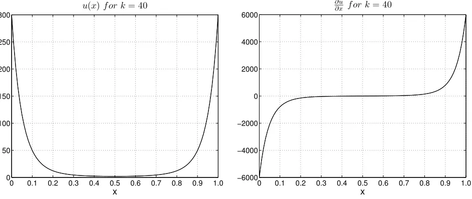
showing the formation of shock structures at each side of the problem domain. The decay parameter k in the convective velocity corresponds to the scale of shock structures at the problem boundaries. In this work we consider k = 40, and in order to obtain a symmetric shock structures at both sides of the domain the same value of the potential is prescribed at the inlet and outlet of the problem domain, U0=U1= 300. For more details see Fig. 1, where the analytical solution of the potential function and
its longitudinal derivative for the case ofk= 40 are reported.
0 0.1 0.2 0.3 0.4 0.5 0.6 0.7 0.8 0.9 1.0 0
50 100 150 200 250 300
x u(x)for k= 40
0 0.1 0.2 0.3 0.4 0.5 0.6 0.7 0.8 0.9 1.0 −6000
−4000 −2000 0 2000 4000 6000
x ∂u
[image:7.595.79.550.172.371.2]∂x for k= 40
Figure 1: Analytical solution of the potential function (left) and its longitudinal derivative (right)
In both cases, CS and GF, the domain is divided into a uniform distribution of massive overlapping rectangular interpolation stencils having one circular integration subregion per stencil, i.e. the number of interpolation stencils is equal to the number of integration subregions. To construct the stencils, a uniform distribution of points is spread over the problem domain and at each of these points a (n×n) stencil is built, containing the stencil centre point and its (2n−1) neighbours. Although better distribution of stencils is always feasible, for the purpose of this comparison this uniform distribution is the most simple and clear way of presenting it. As a refinement strategy to improve the accuracy of the solution, the density of interpolation stencils can be increased and keeping only one collocation point per integration subregion, which is equivalent to a mesh refinement. Alternatively, it is possible to keep the original uniform distribution of stencils but increase the number of collocation points at the integration subregions, as required. This second alternative is only possible to be considered when using the GF and not when using the CS. This last approach will be used to show the limitations of using the CS instead of the complete GF.
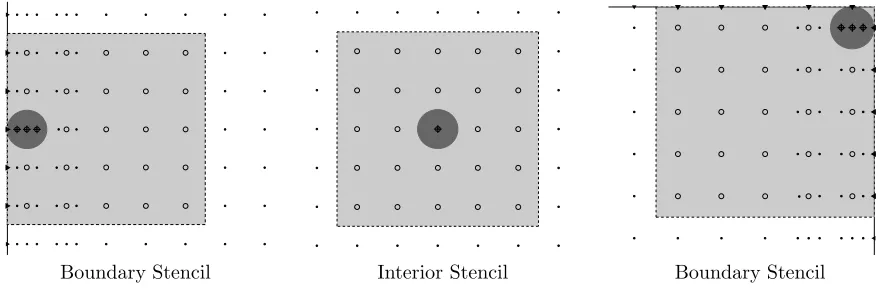
In the case of the CS, where only one source point is included per stencil, the number of interpolation stencils, Nis, is equal to the number of collocation points (Nsp). In this work when using this type of function (CS), we only employ stencils with 25 interpolation points, n = 5, where the stencil’s center is included, i.e. the integral collocation point, see Fig. 2 for the schematic representation of the stencil configuration around the computational domain where the circles represent the corresponding integration subregions.
and not the source points of the integration subregion of the neighbouring interpolation points in the stencil, which corespond to the integration on the overlapped stencils. Therefore in our case, we have stencils with 25 interpolation points at the center of the domain and with 27 points at each lateral side of the domain. In this way, the number of integration subregions (interpolation stencils),Nis, is smaller than the number of collocation points,Nsp, since in those stencils with 27 points we have the additional two collocation points per integration subregion (see Fig. 3 for the corresponding stencil configuration and integration collocation points around the computational domain).
[image:8.595.78.527.179.333.2]Boundary Stencil Interior Stencil Boundary Stencil
Figure 2: Stencil configuration. Regular Distribution
Boundary Stencil Interior Stencil Boundary Stencil
Figure 3: Stencil configuration. P-adaptive Distribution
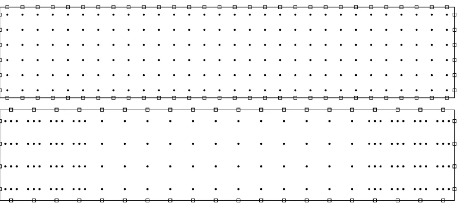
A schematic representation of the source points distribution over the computational domain for the two cases mentioned above can be seen in Fig. 4, where the illustration at the top corresponds to the CS and at the bottom to the GF, with the P-adaptive distribution of source points (integral collocation points) towards the shock structures.
[image:8.595.80.519.385.529.2]Figure 4: Schematic representation of source points distributions
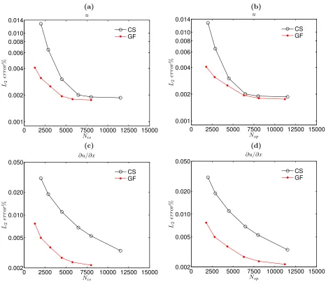
In the table, the L2 error norms for u and ∂u/∂x are reported, where the reconstruction of the derivative was obtained via the differentiation of the integral equation (10) at the center point of each integration subregion. As can be observed from the table, for similar numbers of source points,Nsp, both results show the same order of approximation, being the results with the GF P-adaptive distribution of source points always slightly better, in particular in the estimation of the derivative. However, looking at the number of interpolation stencils (integration subregions), Nis, the GF results always require a significantly lower number of stencils than those used by the CS to achieve a similar accuracy; for example the CS result forNis= 8000 attains a L2 error norm of 1.9E-03 foruand of 5.28E-03 for∂u/∂x while the GF results require onlyNis= 4500 to reach a L2 error norm of 1.93E-3 foruand of 2.71E-03 for∂u/∂x, with always better precision on the derivative. This behaviour is illustrated in Figure 5, where we compare the performance of CS and GF by plotting the uand ∂u/∂x L2 error norms for different numbers of integration subregions, Nis, and source points,Nsp. Subfigures (a) and (b) show numerical results for the concentration against Nis and Nsp, respectively. Similar results for ∂u/∂x are shown in subfigures (c) and (d).
The main point to address here is the P-adaptive character of the general use of the GF, with the possibility of more than one source point per integration subregion. By looking at the results in Table 1, it can be observed that when using the CS with a uniform distribution ofNis= 4500 integration circles (equal to the number of interpolation stencils) with only one source point per circle at their centres, Nsp = 4500, results in a L2 error norm of 3.0E-3 for uand of 1.1E-02 for ∂u/∂x. On the other hand, when the number of source points are increased in the regions of high gradient of the solution (shock structures) to a total number ofNsp= 6300, by using the P-adaptive character of the GF, and keeping the same number of integration circles (Nsp= 4500), the L2 error norm of the result reduces to 1.94E-3 foruand to 2.71E-03 for∂u/∂x, with a gain of one order of magnitude on the estimation of the derivative.
3.1
Results for different sizes of integration subregion
Companion Solution (CS) Green’s function (GF) Regular distribution P-adaptive distribution
Nis Nsp L2−Error%u L2−Error%∂u/∂x Nis Nsp L2−Error%u L2−Error%∂u/∂x
[image:10.595.79.551.84.187.2]2000 2000 1,2725E-02 3.0579E-02 1280 1792 4.0688E-03 7.6900E-03 2880 2880 6.4989E-03 1.8826E-02 2000 2800 3.1114E-03 4.9836E-03 4500 4500 3.0147E-03 1.1006E-02 3125 4325 2.5049E-03 3.7308E-03 6480 6480 2.0047E-03 6.8181E-03 4500 6300 1.9385E-03 2.7126E-03 8000 8000 1.9039E-03 5.2833E-03 5780 8092 1.7984E-03 2.3728E-03 11520 11520 1.8644E-03 3.3706E-03 8000 11200 1.7570E-03 2.1694E-03
Table 1: L2 error norm foruand∂u/∂x: Companion Solution (Regular distribution) Vs Green’s function (P-adaptive distribution). Nis: number of integration subregions. Nsp: number of source points.
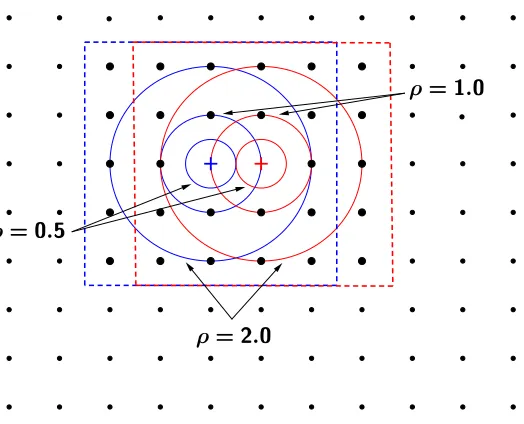
to ρ= 0.5,ρ= 1 and 2. For values of ρ >0.5 the integration circles will partially overlap each other, according to the position of the overlapping stencils considered.
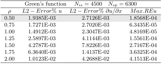
In Table 2, results for seven different values ofρare presented, ranging from 0.5 to 2, for the P-adaptive domain discretization corresponding to 4500 integration subregions and 6300 source points. The results in the shaded row of the table correspond to those of the shaded row in Table 1, forρ= 0.5,Nis= 4500 andNsp= 6300. As can be seen from these results, the L2 error norm of the potential and its derivative are all of the same order of magnitude until ρ= 1.50, with the best solution obtained for ρ= 1.0 also having the smaller maximum relative error. When ρ = 0.5 all the circles belonging to the boundary interpolation stencils are tangential to the problem boundary, see figures 6, 2 and 3. On the other hand, values of ρ >0.5 implies overlapping that corresponds in our implementation to some level of extrapo-lation at the boundary interpoextrapo-lation stencils in order to evaluate the double layer potential density uat the part of the circles outside the problem domain. Extrapolation is a bad mathematical operator and too much extrapolation will deteriorate the results, as happens forρ >1.0 when the solution start to lose accuracy.
Green’s function Nis= 4500 Nsp= 6300 ρ L2−Error%u L2−Error%∂u/∂x M ax.REu
0.50 1.9385E-03 2.7126E-03 1.8568E-04 0.75 1.7271E-03 2.7020E-03 6.3435E-05 1.00 1.4912E-03 2.3047E-03 4.8169E-05 1.25 2.5897E-03 4.1144E-03 1.5561E-04 1.50 4.2787E-03 7.8226E-03 2.7167E-04 1.75 6.3640E-03 1.4137E-02 3.6325E-04 2.00 1.0123E-02 4.2688E-02 4.1513E-04
Table 2: Numerical results for different sizes of the integration subregion
4
Conclusions
[image:10.595.169.427.438.541.2](a) (b)
0 2500 5000 7500 10000 12500 15000
0.001 0.002 0.004 0.006 0.008 0.010 0.014 Nis L2 er ro r % u CS GF
0 2500 5000 7500 10000 12500 15000
0.001 0.002 0.004 0.006 0.008 0.010 0.014 Nsp L2 er ro r % u CS GF (c) (d)
0 2500 5000 7500 10000 12500 15000
0.002 0.005 0.010 0.020 0.050 Nis L2 er ro r % ∂u/∂x CS GF
0 2500 5000 7500 10000 12500 15000
[image:11.595.76.542.82.489.2]0.002 0.005 0.010 0.020 0.050 Nsp L2 er ro r % ∂u/∂x CS GF
Figure 5: Variation of L2 error norms foruand ∂u/∂x, with the number of integration subregions and source points
to implement the proposed P-adaptive scheme in order to improve the accuracy of the numerical solution without increasing the number of integration subregions, as shown in the results reported in figure 5. In the case of having only one collocation point per integration subregion, it is also possible to improve locally the accuracy of the solution by increasing the number of integration subregions at computational complex regions, in a type of h-adaptive scheme. However, when using the complete form of the Dirichlet Green’s function both approaches can be used simultaneously, i.e. h and P-adaptive, by increasing the number of integration subregions and the number of collocation points at the required subregions.
Everything addressed here for two dimensional problems is identically valid for the corresponding three dimensional analogous cases, as well as the analysis presented for the Laplace equation is valid for any other well posed boundary (initial) value problem having a fundamental solution. Different analytical approaches are available in the literature to find the Dirichlet Green’s function on a circle or a sphere for different partial differential equations, most of them based on the equivalent circle or sphere theorems, see Maul and Kim [9] and Kukla et al. [8] for the corresponding Dirichlet Green’s functions for the Stokes system of equations and Helmholtz equation, respectively.
Figure 6: Stencils with different sizes of integration subregions
or mixed type boundary conditions. In this way, it is possible to use always circular or spherical integration contours even in regions near or in contact with the problem domain, where the densities of the integrals, i.e. the corresponding values of the field variables at the integration contours, are reconstructed from the interpolation formulae that already included the problem boundary conditions. It is also shown that it is possible to use overlapping or non-overlapping integration subregions as long as overlapping interpolation stencils are employed. In the case of using everywhere overlapping circular integration contours, the proposed meshless scheme implies some level of extrapolation at the boundary interpolation stencils in order to evaluate the double layer potential density at the part of the circles outside the problem domain. It was found that a more accurate solution is obtained when only small extrapolation is allowed, see table 2. This is due to the fact that extrapolation is a bad mathematical operator and too much extrapolation will deteriorate the results. However, some extrapolation is desirable, but not necessary, to be able to cover all the problem domain with the integrations subregions. A major consequence of using circular integration contours everywhere in the problem domain is that is not necessary to truncate the integration contours at intersections with the problem boundary, with the problem boundary conditions implemented at those parts of integration contours coinciding with the problem domain instead of being considered at the corresponding interpolation stencils as proposed in our meshless implementation. Besides by using truncated circular integration contours at the problem boundary, it is always necessary to evaluate part of the single layer potential at those common integration surfaces with the problem boundary. On the other hand, in the case of using circular integration contours everywhere and imposing the boundary conditions at the level of the interpolation algorithm instead of at the integral representation formula (as considered here), the singular layer potential is always eliminated by the use of the Dirichlet Green’s function for a circular domain.
References
[1] Askin, S., and Fenner, R. T. Applications of the local boundary integral equation technique to potential problems. Applied Mathematical Modelling 17 ISSN:0307-904X (1993), 246–245.
[3] Caruso, N., Portapila, M., and Power, H. An efficient and accurate implementation of the localized regular dual reciprocity method.Computers and Mathematics with Applications 69 (2015), 1342–1366.
[4] Dehghan, M., and Shirzadi, M. A meshless method based on the dual reciprocity method for one-dimensional stochastic partial differential equations. Numerical Methods for Partial Differential Equations 32, 1 (2016), 292–306.
[5] J. Sladek, V. S., and Atluri, S. N. Local boundary integral equation (lbie) method for solving problems of elasticity with nonhomogeneous material properties. Computational Mechanics 24(6) (2000), 479–496.
[6] J. Sladek, V. S., and Zhang, C. A local biem for analysis of transient heat conduction with nonlinear source terms in fgms. Engineering Analysis with Boundary Elements 28 (2004), 1–11.
[7] Kov´aˇr´ık, K., Muˇz´ık, J., and Mahmood, M. A meshless solution of two-dimensional unsteady flow. Engineering Analysis with Boundary Elements 36, 5 (2012), 738 – 743.
[8] Kukla, S., Siedlecka, U., and Zamorska, I. Green’s functions for interior and exterior helmholtz problems. Scientific Research of the Institute of Mathematics and Computer Science 11(1) (2012), 53–62.
[9] Maul, C., and Kim, S. Image of a point force in a spherical container and its connection to the Lorentz reflection formula. Journal of Engineering Mathematics 30, 1 (1996), 119–130.
[10] Milne-Thomson, L. M. Theoretical Hydrodynamics. The Macmillan Company, New York, 1968.
[11] Popov, V., and Bui, T. T. A meshless solution to two-dimensional convection-diffusion problems. Engineering Analysis with Boundary Elements 34 (2010), 680–689.
[12] Popov, V., and Power, H. The DRM-MD integral equation method: an efficent approach for the numerical solution of domain dominant problems. International Jounal for Numerical Methods in Enginerering 44 (1999), 327–353.
[13] Portapila, M., and Power, H. A convergence analysis of the performance of the DRM-MD boundary integral approach.International Journal for Numerical Methods in Engineering 71 (2007), 47–65.
[14] Portapila, M., and Power, H. Iterative solution schemes for quadratic DRM-MD. Numerical Methods for Partial Differential Equations 24(6) (2008), 1430–1459.
[15] S. N. Atluri, H. G. K., and Cho, J. Y. A critical assessment of the truly meshless local petrov-galerkin (mlpg), and local boundary integral equation (lbie) methods. Computational Mechanics 24(5) (1999), 348–372.
[16] Sellountos, E. J., Polyzos, D., and Atluri, S. N. A new and simple meshless LBIE-RBF numerical scheme in linear elasticit. Computer Modeling in Engineering adn Sciences 89(6) (2012), 513–551.
[17] Sladek, J., Sladek, V., and Zhang, C.A meshless local boundary integral equation method for heat conduction analysis in nonhomogeneous solids. Journal of the Chinese Institute of Engineers 27, 4 (2004), 517–539.
[18] Taigbenu, A. E. The green element method. International Journal for Numerical Methods in Engineering 38(13) (1995), 2241–2263.