March 21, 2017
Contribution of mode-coupling and phase-mixing of Alfvén waves
to coronal heating
P. Pagano
1and I. De Moortel
1School of Mathematics and Statistics, University of St Andrews, North Haugh, St Andrews, Fife, Scotland KY16 9SS, UK. e-mail: [email protected]
ABSTRACT
Context.Phase-mixing of Alfvén waves in the solar corona has been identified as one possible candidate to explain coronal heating. While this scenario is supported by observations of ubiquitous oscillations in the corona carrying sufficient wave energy and by theoretical models that have described the concentration of energy in small-scale structures, it is still unclear whether this wave energy can be converted into thermal energy in order to maintain the million-degree hot solar corona.
Aims.The aim of this work is to assess how much energy can be converted into thermal energy by a phase-mixing process triggered by the propagation of Alfvénic waves in a cylindric coronal structure, such as a coronal loop, and to estimate the impact of this conversion on the coronal heating and thermal structure of the solar corona.
Methods.To this end, we ran 3D MHD simulations of a magnetised cylinder where the Alfvén speed varies through a boundary shell, and a footpoint driver is set to trigger kink modes that mode couple to torsional Alfvén modes in the boundary shell. These Alfvén waves are expected to phase-mix, and the system allows us to study the subsequent thermal energy deposition. We ran a reference simulation to explain the main process and then we varied the simulation parameters, such as the size of the boundary shell, its structure, and the persistence of the driver.
Results.When we take high values of magnetic resistivity and strong footpoint drivers into consideration, we find that i) phase-mixing leads to a temperature increase of the order of 105K or less, depending on the structure of the boundary shell, ii) this energy is able to balance the radiative losses only in the localised region involved in the heating, and iii) we can determine the influence of the boundary layer and the persistence of the driver on the thermal structure of the system.
Conclusions.Our conclusion is that as a result of the extreme physical parameters we adopted and the moderate impact on the heating of the system, it is unlikely that phase-mixing can contribute on a global scale to the heating of the solar corona.
Key words.
1. Introduction
The coronal heating has been an unsolved problem for several decades, and the mechanism behind the million-degree hot so-lar corona is still unclear. Of course, all this time has not been passed idly, and different generations of instruments and models have brought further insights to the problem. We recommend De Moortel & Browning (2015) and references therein for a com-prehensive review.
One of the candidates suggested to explain coronal heating is phase-mixing of Alfvén waves (Heyvaerts & Priest 1983), which is one of the main models where Alfvén waves are put forward to explain the thermal structure of the solar corona. (see Arregui 2015, for a more extended review). In this specific model, lo-calised small-scale gradients develop when Alfvén waves prop-agate at different speeds and these are preferred locations where magnetic and kinetic energy can be converted into heating. Re-cently, this model has fallen under careful scrutiny from the coronal physics community because theoretical results and ob-servations have opened the possibility for phase-mixing to ex-plain coronal heating (e.g. Cargill et al. 2016).
Oscillations in the solar corona have been observed for more than a decade, and some studies have suggested that the damping of waves could be connected with coronal heating (Nakariakov et al. 1999). However, observations of ubiquitous Alfvén waves have only more recently concluded that waves carry enough
en-ergy to account for the coronal heating (Tomczyk et al. 2007; Jess et al. 2009; McIntosh et al. 2011), where wave disturbances are sufficiently intense to power the quiet Sun and coronal holes, while active regions remain offthe range by an order of magni-tude (see also De Moortel & Nakariakov 2012, for a more com-prehensive review). Morton & McLaughlin (2013) focused on low-amplitude oscillations, where the authors found that wave activity is low over an extended period of time, and these os-cillations would not be able to match the energy requirements of active regions. Threlfall et al. (2013) identified unambigu-ous wave propagations by simultaneunambigu-ously measuring the veloc-ity and displacement of observed coronal loops that López Ariste et al. (2015) have interpreted as combined propagation of kink and sausage wave modes.
Pascoe et al. (2016) observed and analysed the damping of some coronal loop oscillations by making a detailed seismologic anal-ysis to retrive the loop parameters, while Goddard et al. (2016) examined a large set of kink oscillations to carry out a statisti-cal study on how these oscillations undergo damping in the so-lar corona. Additionally, other studies have compared observed heating properties with models in order to constrain the models. Van Doorsselaere et al. (2007) found that coronal loop heating profiles match a resistive wave heating mechanism better than a viscous one. Okamoto et al. (2015) observed the oscillations of threads of a coronal prominence, identified as standing Alfvén waves, and their subsequent damping, and Antolin et al. (2015) argued that the observed damping of the oscillations is enhanced by the development of Kelvin-Helmotz instabilities at the bound-aries of the threads.
On the theoretical side, the highly structured solar corona suggests the presence of numerous interfaces between the many magnetic structures where plasma and magnetic field vary and offers the ideal environment where Alfvén waves can propagate at different speeds. At the same time, such coronal structures are anchored to the base of the corona where footpoints move hori-zontally as a result of photospheric and chromospheric motions, which means that they move transversally to the magnetic field and are likely to cause phase-mixing of transverse waves. In this context, the magnetohydrodynamical (MHD) numerical experi-ments of Pascoe et al. (2010), Pascoe et al. (2011), Pascoe et al. (2012), and Pascoe et al. (2013) have shown that phase-mixing can be triggered in the solar corona when kink oscillations of coronal loops lead to the propagation of Alfvénic waves along the inhomogeneous flux tube. It has been reliably proven that this process leads to the concentration of wave energy in the in-homogeneous boundary shell and the formation of small-scale structures. This model has also described that the structures gen-erated by the phase-mixing on the boundary shell become in-creasingly smaller. This result has been validated in different and increasingly realistic configurations, and it has been con-cluded that this energy eventually needs to be dissipated. Earlier on, ideal MHD simulations by Poedts & Boynton (1996) had es-timated the heating that is due to phase-mixing of Alfvén waves propagating along a magnetised cylinder by assuming turbulent heating following the ideal evolution. Soler et al. (2016) ran a similar analysis of propagating Alfvén waves in prominences, but approached the problem from an analytical point of view and also estimated the heating that can derive from this process. They found that wave heating can contribute a fraction of the radiative losses and only under certain conditions.
These data and numerical experiments have opened up the possibility that the damping of kink oscillations could contribute to the coronal heating, and with this premise, phase-mixing is a likely candidate mechanism that could enhance the damping of waves and lead to the conversion into coronal heating. The aim of this work is therefore to test this hypothesis and to assess the possible contribution to coronal heating that can derive from the damping of kink waves through phase-mixing.
[image:2.612.362.505.10.289.2]To this end, we continue the study of Pascoe et al. (2010), where MHD simulations of a magnetised cylinder with the pres-ence of a driver at one of the footpoints are used to simulate the propagation of a kink mode in a coronal loop and the subsequent mode-coupling with the (m = 1) Alfvén mode of the loop and dissipation of these waves through phase-mixing. In our simula-tions we also account for non-ideal terms such as magnetic re-sistivity and thermal condution in order to investigate how much energy is converted into heating and how the plasma temper-ature changes following this process. To do so, we first run a
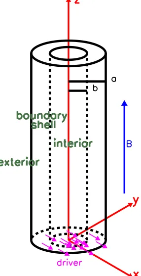
Fig. 1. Sketch to illustrate the geometry of our system and the Cartesian axes.
reference MHD simulation where a single pulse driver is set in, and we analyse the energy deposition in the boundary shell. We then run a series of simulations where we investigate the role of the width and shape of the boundary shell, and how the results change when a continuous driver acts instead of a single pulse.
The paper is structured as follows: in Sect. 2 we describe our reference model, in Sect. 3 we analyse our reference simulation in full detail, in Sect. 4 we vary some properties of the boundary shell and the driver, and in Sect. 5 we discuss our results and draw some conclusions.
2. Model
In order to investigate the deposition of thermal energy in the solar corona during the mode-coupling and phase-mixing, we devise a numerical experiment following the same pattern as in-troduced by Pascoe et al. (2010), Pascoe et al. (2011), and Pascoe et al. (2012).
2.1. Initial condition
We consider a cylindrical flux tube where we define an interior region, a boundary shell, and an exterior region (Fig. 1). The system is set in a Cartesian reference frame with z being the direction along the cylinder axis, and x and y define the plane across the cylinder section. The origin of the axes is placed at the centre of one footpoint of the cylinder. The cylinder has radius a, the interior region has radius b,and the boundary shell covers a fraction l=(a−b)/a of the cylinder radius. The boundary shell
is the ring between radii b and a, and the exterior region is the rest of the domain beyond radius a.
Table 1. Parameters
Parameter value Units
a 1 Mm
l 0.5 a
ρi 1.16×10⁻¹⁶ g/cm3 ρe 2.32×10⁻¹⁶ g/cm3
T0 1.58 MK
Be 6.18 G
a, and b:
ρ(ρe, ρi,a,b)=ρe+
ρi−ρe
2
"
1−tanh e a−b
"
r−b+a 2
#!# ,
(1)
where r = px2+y2 is the radial distance from the centre of the cylinder, ρe is the density in the exterior region, and ρi is the density in the interior. The temperature of the plasma, T , is assumed uniform at T0, and the thermal pressure, p, is set by the equation of state
p= ρ
0.5mp
kbT, (2)
where mpis the proton mass and kb is the Boltzmann constant. The flux tube is initially in equilibrium, and in order to allow the propagation of kink waves and provide magnetohydrostatic equilibrium, we set a non-uniform magnetic field, B, along the
z-direction:
Bz=
q
B2
e−2(p−pe), (3)
which balances the varying thermal pressure, where Be is the value of the field in the exterior region, peis the thermal pressure in the exterior region (derived fromρeand T0), and p is the local value of the thermal pressure. In Table 1 we list the values of the free parameters used to set up our specific experiment.
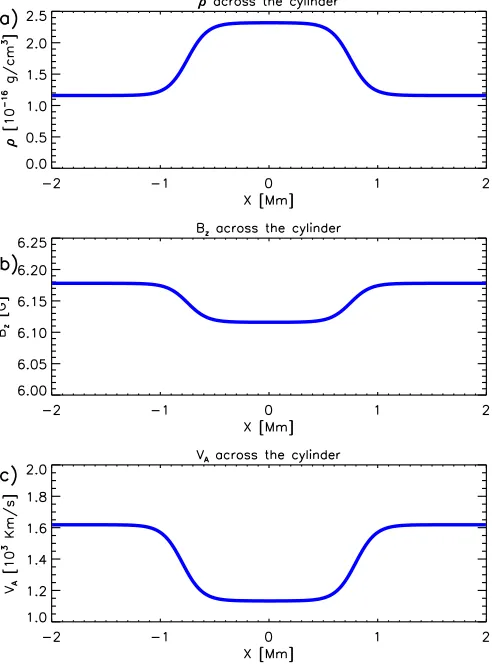
Figure 2 shows the value of ρ, Bz, and the corresponding Alfvén speed (VA) across the cylinder. In particular, VAis higher in the exterior region and decreases in the boundary shell, where the maximum gradient is at r ≃0.8a. With the present parame-ters, the plasmaβis uniformlyβ=0.02.
2.2. Driver
A driver acts on the system in order to initiate the propaga-tion of Alfvénic waves within the system (represented in pink in our sketch in Fig. 1). The driver is prescribed by the displace-ment along the x-axis of the flux tube below the lower z bound-ary of the cylinder and by the consequent velocity perturbation. Specifically, Fig. 3a (blue line) shows the position of the centre of the flux tube as a function of time, whose expression is given by
s(t)= V0
ω sinωt sin ωt
2 , (4)
where V0 is the amplitude of the speed of the displacement, ω =2π/P is the angular frequency derived by the period of the
oscillations P, and V0/ωis the following spatial displacement of the centre of the flux tube. The driver sets in at t =0 and stops at t = P. This displacement of the flux tube leads to a uniform
velocity perturbation within the interior region and the boundary
Fig. 2. Cuts of our initial condition for our MHD model across the cylin-der. (a) Density, (b) z−component of the magnetic field, and (c) Alfvén speed.
shell that is described by the time derivative of Eq. 4 (Fig. 3a, red line):
vx0= ds(t)
dt =V0
cosωt sinωt
2 +0.5 sinωt cos ωt
2
. (5)
As in Pascoe et al. (2011), this choice for the driver combines an oscillatory motion at the footpoint (∼sin(ωt)) with an envelope
of sin(ω/2t) to ensure a smooth (continuous) acceleration at t= 0. In the exterior region, we assume that the system reacts to the flux tube motion as a 2D dipole velocity configuration, so that the x and y components of the velocity in the exterior region can be written as a function of time and space as
vx=vx0a2
(x2−y2)
(x2+y2)2 (6)
vy=vx0a2 2xy
(x2+y2)2. (7)
This choice allows a smooth transition between the boundary shell and the exterior region as the velocity amplitude is never discontinuous and mimics plasma flows around the magnetised cylinder when in motion. Figure 3b shows the driver configura-tion at t=P/2 when the velocity is maximum and the flux tube is at its rest position. Table 2 summarises the values we used to set up the driver in our numerical experiment.
Fig. 3. Settings for the driver. (a) Time evolution of the cylinder centre footpoint displacement as a function of time (blue line) and the con-sequent velocity displacement (red line). (b) Map of the density of the driver at t=0.5 P with the velocity arrow overplotted. The maximum velocity in the cylinder at this time is V0, according to Table 2.
Table 2. Parameters
Parameter value Units
V0 113 km/s
P 6.18 s
usually considered horizontal footpoint motions (Threlfall et al. 2013). The period of the driver is designed to produce a visible effect on the present numerical experiment and is not meant to represent a significant frequency in the power spectrum of the corona. At the same time, while the period is well below the peak of the 5 minutes, oscillations of the order of seconds could still contribute to the power spectrum of the velocity perturbation at the coronal footpoints.
2.3. MHD simulation
In order to study the evolution of the system caused by the foot-point driver, we used the MPI-AMRVAC software (Porth et al. 2014) to solve the MHD equations, where thermal conduction,
magnetic diffusion, and joule heating are treated as source terms:
∂ρ
∂t +∇·(ρv)=0, (8)
∂ρv
∂t +∇·(ρvv)+∇p−
j×B
c =0, (9)
∂B
∂t −∇×(v×B)=η c2 4π∇
2B, (10)
∂e
∂t +∇·[(e+p)v]=−ηj
2− ∇ ·F
c, (11)
where t is time, v velocity,ηthe magnetic resistivity, c the speed of light, j= 4πc∇ ×B the current density, and Fcthe conductive flux (Spitzer 1962). The total energy density e is given by
e= p
γ−1 + 1 2ρv
2+ B 2
8π, (12)
whereγ=5/3 denotes the ratio of specific heats.
In our numerical experiments we adopted a value ofηthat is set uniformly asη = 109ηS , whereηS is the classical value at T =2 MK (Spitzer 1962).
The computational domain is composed of 512×256×512 cells, distributed on a uniform grid. The simulation domain ex-tends from x = −2 Mm to x = 2 Mm, from y = −2 Mm to
y=0 Mm (where we model only half of a flux tube) and from
z=0 Mm to z=40 Mm in the direction of the initial magnetic field. The boundary conditions are treated with a system of ghost cells, and we have periodic boundary conditions at both x bound-aries, reflective boundary conditions at the y boundary crossing the centre of the flux tube, and outflow boundary conditions at the other y boundary. The driver is set as a boundary condition at the lower z boundary and outflow boundary conditions are set at the upper z boundary.
3. Reference simulation
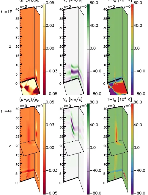
The evolution of the MHD simulation allows us to analyse how the process of mocoupling and phase-mixing leads to the de-position of thermal energy in the system. As soon as the driver sets in, a wavetrain propagates into the domain, and we illustrate the evolution that follows in Fig. 4, where we show maps of den-sity contrast (ρ(t)−ρ(0))/ρ(0), the x-component of the velocity and temperature of the plasma at t=P and t=4 P in a projec-tion of the 3D simulaprojec-tion box where we cut two vertical planes at x=0 and y=0 and a horizontal plane at the z coordinates of the trail of the wavetrain propagating at the Alfvén speed of the interior region.
The evolution described by the y =0 plane is the expected evolution of an oscillation of the flux tube along the x direction, where we see weak compression and rarefaction according to the phase of the driver, alternating positive and negative vxregions, and no significant temperature change. Additionally, an acoustic mode follows the propagation of the transverse wave and leads to a visible compression and rarefaction at z=5 Mm at t=4P.
Fig. 4. 3D cuts of the MHD simulation where show maps of density contrast (ρ(t)−ρ(0))/ρ(0) (left column), vx(centre column), and
tem-perature change (T (t)−T (0)) (right column) on the x =0 and y =0 plane and the horizontal plane at the z=(t−P)VA0coordinate at t=1 P (upper row) and t=4 P (lower row).
As the purpose of this work is to identify the capacity of these phenomena to convert the magnetic and kinetic energy concen-trated in the boundary shell into plasma heating, we address the temperature change in the boundary shell at t=4P (Fig. 4 right column). We find that a region of increased temperature along the vertical direction inside the boundary shell is formed. This region has a slightly variable width and extends over about 45◦ on the xy plane, as we see in the horizontal cut at t=4 P. In this simulation the heating is of the order to 5×10⁴ K and reaches 7×10⁴K in some regions.
Figure 5a shows the temperature increase profile at z=26.60
Mm from t=3.2 P to t=5 P with a cadence of 0.1 P (from the thinnest to the thickest line) where the red vertical line marks the position of the maximum gradient of the Alfvén speed. The temperature starts to increase in the boundary shell near its bor-der with the exterior region, where the kinetic energy is higher. Then the temperature increase profile maximum drifts towards the centre of the boundary shell and stops at the position where the gradient of the Alfvén speed is maximum, and from there it develops in a temperature increase profile centred at that po-sition. The green line in Fig. 5a follows the maximum of the temperature increase that approaches the centre of the bound-ary shell in three consecutive segments, each determined by the arrival of one of the velocity peaks induced by the driver. The location of the maximum gradient of the Alfvén speed does not change over this time frame. Figure 5b stacks cuts of the
temper-Fig. 5. Temperature difference (T (t)−T (0)) cuts. (a) Cuts at x = 0 and z=26.6 Mm (where the maximum temperature is found) between t =3.2 P (thinnest line) and t = 5 P (thickest line). The vertical red dashed lines are the borders of the boundary shell, and the red lines are placed at the location of the maximum gradient of the Alfvén speed at each time. (b) Staggered cuts along the z direction on the x=0 at the initial location of the maximum gradient of the Alfvén speed. The green line follows the location of the maximum temperature increase in both plots.
ature increase along the z-direction at different times every 0.1P at the y coordinate where the maximum of the gradient of the Alfvén speed is situated. We note that the bump in the temper-ature increase is located at higher z as the evolution progresses until t =4 P, when it settles at about z=27 Mm. At the same time, its magnitude increases as well. At t =5P the maximum temperature increase is 7×10⁴K. It should also be noted that at each time the maximum temperature increase lags the perturba-tion, as is visible from the wave that propagates from the origin towards the edge of the domain.
Similar conclusions can be made based on Fig. 6, where we show maps of the quantity∇2B
x (Fig. 6a) and temperature in-crease (Fig. 6b) at t =4P on the x=0 plane. The black arrows represent the Poynting flux (only where its intensity is above a threshold), and we chose∇2Bxbecause it is some order of mag-nitude larger than∇2Byand∇2Bz. As we are investigating a non-ideal heating mechanism, we focus on∇2B
xbecause where this term is large, magnetic diffusivity operates and magnetic energy is converted into heating. Where∇2B
[image:5.612.309.557.11.306.2]Fig. 6. Maps on the x=0 plane of (a)∇2B
xand (b) the temperature
[image:6.612.317.554.8.258.2]dif-ference (T (t)−T (0)) at t=4 P with Poynting flux vectors overplotted where this is more intense. In panel (a) the dashed blue lines define the borders of the boundary shell.
Fig. 7. Temperature difference evolution of two points on the x = 0 plane at the location of the maximum gradient of the Alfvén speed at z= 26.60 Mm (red line, where the maximum temperature in the simulation is reached at t=5 P) and at z=13.32 Mm (blue line).
has occurred, together with the formation of regions with high ∇2B
x.
Additionally, the heating takes place over a bounded pe-riod of time from when the phase-mixing starts to occur until the process of conversion of energy into thermal energy is con-cluded. Figure 7 shows the temperature evolution of two points at z = 13.32 Mm (blue line) and z = 26.60 Mm (red line) at the x =0 plane at the location of the maximum gradient of the Alfvén speed. The vertical lines show the time at which a wave that propagates from the lower boundary at the Alfvén speed of the exterior region reaches the two points (fronts), and the time at which a wave that propagates from the lower boundary when the driver ends at the speed of the Alfvén speed of the interior region (trails). The temperature remains constant as long as no perturbation reaches the point, it then steadily increases as the energy concentrated in the boundary shell is dissipated, and it finally remains constant again. While this evolution is common for both points, the final temperature depends on the z coordi-nate because the amount of energy that can be converted into heating depends on the intensity of the gradients of the
mag-Fig. 8. (a) Difference in energy in the boundary shell between time t and t = 1 P: magnetic (blue lines - Bx, magenta lines - Bz), kinetic
(green lines), and thermal (red lines) energy for the simulations with
η = 109η
S andη = 0. (b) Difference in the energy in the boundary
shell between the simulation withη=109η
S andη=0 normalized to
the thermal energy difference between the two simulations at each time. Note that the horizontal axis in both panels starts at t=1 P, i.e. when the boundary driving has terminated.
netic field, which become steeper in z the more out of phase adjacent propagating waves are. At the same time, because of the progressive damping of waves, there is more kinetic energy available at lower z-coordinates than higher up. In the present analysis the time integral of the kinetic energy in the boundary shell that crosses the z=13.32 Mm surface is 20% higher than the time integral of the kinetic energy that crosses the z=26.60
Mm.
In order to further investigate how the energy is converted into heating, we ran a simulation where we set η = 0 to ex-clude the resistivity effects. In MHD simulation terms, this cor-responds to adopting numerical resistivity, which is the lowest resistivity value that a given MHD simulation can achieve. The simulation withη=0 shows an evolution very similar to the one in Sect. 3, except that no significant temperature increase occurs through phase-mixing (lower than 5×10³K).
Figure 8a shows the change in magnetic energy (associated with B2xand B2z), kinetic, and thermal energy in the boundary shell compared to the time t =P (when the driver has stopped)
as a function of time in the two simulations. The magnetic en-ergy associated with B2
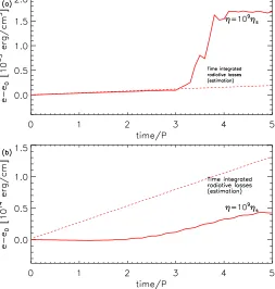
[image:6.612.50.295.263.424.2]Fig. 9. Thermal energy difference as a function of time (a) in the same point as in Fig.7 at z=26.60 Mm and (b) integrated in the entire x=0 plane. The red dashed line in both plots is an estimate of the radiative losses for the region of interest.
the driver-induced transverse wave motions, as the equilibrium magnetic field is not constant in the domain. This analysis shows again that the non-ideal MHD terms are essential to convert the energy concentrated in the boundary shell into heating. In Fig. 8b we set equal to 1 the difference of the thermal energy in the boundary shell at any given time between the simulation with resistivity and the one without. The corresponding difference in magnetic (Bx) and kinetic energy is about the same, at a value of−0.6. This result suggests that the kinetic and magnetic en-ergy contribute to the same extent in providing the system with thermal energy, as expected for Alfvén waves and predicted in Heyvaerts & Priest (1983).
However, the open question is whether this energy input can match the radiative losses in order to answer to which extent this heating mechanism can contribute to the coronal heating. In Fig. 9a we show the internal energy evolution in a plasma element located on the phase-mixing shell at z = 26.60 Mm (same as red line in Fig.7) as a function of time compared with an esti-mate of the cumulated radiative losses following from the den-sity and temperature evolution of the same plasma element. We find that the energy deposition in a single plasma element can largely overcome the radiative losses. However, the question is not whether the heating mechanism can maintain coronal tem-perature in a single favourable location, but if it can supply suf-ficient energy for entire coronal structures. Figure 9b shows the result when the same analysis is carried out and integrated on the upper three quarters of the x=0 plane of the present simulation (we exclude the lower part to avoid spurious variations that are due to the lower boundary of the simulation and the propagation of the acoustic mode). As the heating is localised in a narrow re-gion near the phase-mixing shell, the energy contribution to this extended domain is insufficient to balance the energy lost by ra-diation of the plasma on the plane x=0. This spatial domain is
arbitrary and plotted just to show the effect of the spatial limita-tion of the heating. Condilimita-tions would be even less favourable to maintain a coronal temperature in this regime if we considered a 3D domain instead.
4. Investigating the parameter space
In Sect. 3 we have described the mechanism that leads to the de-position of thermal energy in the boundary shell as a result of the phase-mixing of propagating Alfvén waves. Our estimation of the thermal energy contribution from this mechanism seems to be inconclusive as to whether it can definitely overcome the radiative losses. In light of this, it is essential to address the role of the boundary shell in this mechanism in order to assess how much the energy deposition can differ from what we have anal-ysed so far. To do so, we ran simulations where the boundary shell of the cylinder varies in width and where it has a more complex structure.
4.1. Boundary shell width
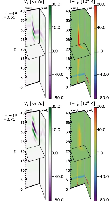
Using the setup explained in Sect. 2, we ran two more simula-tions in which we only changed the width of the boundary shell by using l = 0.75 (wider boundary shell) and l = 0.35 (nar-rower boundary shell) with respect to Table 1. These were anal-ysed in combination with the reference simulation with l =0.5 described in Sect. 3 to investigate how the mode-coupling and phase-mixing are affected by Alfvén speed gradients. A nar-rower boundary shell leads to a steeper Alfvén speed profile (as all other parameters in the setup have remained unchanged), implying that phase-mixing will become more efficient (i.e. the damping length will be shorter Heyvaerts & Priest (1983)). The mode-coupling process that feeds kinetic and magnetic energy into the shell region also depends on the Alfvén speed profile in the shell region, but now a wider shell (a milder Alfvén speed gradient) leads to more efficient mode-coupling (Pascoe et al. 2010, 2012, 2013). Hence, the deposition of thermal energy is dependent on the combined efficiency of mode-coupling and phase-mixing and how the resistivity effects interact with these mechanisms, so that it is not a priori obvious which configuration will be most efficient. The purpose of this experiment is to assess which effect dominates the dynamics and how this influences the non-ideal effects in the simulation, in particular the heating.
Figure 10 shows 3D cuts of vxand T on the x=0 and y=0 planes at t=4 P for the simulations with l=0.35 and l=0.75, to be compared with the simulation with l = 0.5 (Fig.4). The velocity phase-mixing patterns are visibly narrower in the sim-ulation with l = 0.35 and visibly wider in the simulation with
l = 0.75 as they entirely fill the boundary shell. Similar varia-tions are found in the extension of the temperature increase re-gion, where the temperature increase is dependent on the size of the boundary shell, however. The region in which the heating occurs is narrowest in the simulation with l=0.35,and the max-imum temperature increase is∆T ≃105K, while the simulation with l=0.75 show the largest heated region where∆T ≃5×10⁴
K.
Fig. 10. 3D cuts as in Fig. 4 of vx in the left column and temperature
difference, (T (t)−T (0)), right column, at t = 4 P for the simulation with l=0.35 (upper row) and with l=0.75 (lower row).
Fig. 11. Evolution of the wave energy (blue lines) and thermal energy (red lines) in the loop boundary layer as a function of time for different widths of the boundary (l=0.35, dashed line; l=0.50, continuous line; l=0.75, dotted line).
shell region. However, phase-mixing is already taking place at this stage, as is evident from the increase in thermal energy. The thermal energy starts to rise before the wave energy reaches its maximum value. Following this maximum, dissipation through phase-mixing is clearly the dominant process in the shell
re-Fig. 12. Time evolution of the time derivative of the average kinetic energy in the boundary shell (continuous lines) and in the interior region (dashed lines) for the three simulations with l =0.35 (red lines), l = 0.50 (black lines), and l=0.75 (blue lines).
gion: wave energy is converted into thermal energy at a faster rate than it is transferred into the layer by mode-coupling. From comparing the thermal energy curves (red lines), it is clear that the increase in thermal energy is largest for the narrow boundary layer (dashed red line). This is in agreement with Fig. 10, which showed a larger increase in temperature in the boundary layer at t = 4 P for the simulation with the smallest boundary width (l=0.35).
In order to further describe how the width of the boundary shell affects the energy transfer to the boundary shell, we show the time derivative of the average kinetic energy in the interior region and in the boundary shell in Fig. 12. We focus on the av-erage kinetic energy because i) it is the form of energy that is initially pumped into the system and more clearly drifts to the boundary shell, and ii) by averaging over the domain, we com-pensate for two effects: first, the narrower boundary shell simula-tion has more total kinetic energy because it has more plasma in the simulation box, and second, the broader boundary shell sim-ulation has more kinetic energy in the boundary shell because the shell is larger. In Fig. 12 the time derivative is large and pos-itive for t < P while the driver is pumping kinetic energy into
both the interior and boundary shell. After t =1 P,the average kinetic energy in the interior diminishes and it increases in the boundary shell. The time derivative of the average kinetic energy in the interior is negative for all simulations, and the simulation with l=0.75 is the one where it is minimum. The time deriva-tives of the interior region and the boundary shell are opposite in sign, and the total kinetic energy remains roughly constant, with variations of the order of 1%. This confirms that in this first phase the mode-coupling dominates the dynamics, that the ki-netic energy is transferred from the interior to the boundary shell, and that a broader boundary shell makes the energy transfer via mode-coupling more efficient. This phase continues until t∼2.5
[image:8.612.304.560.13.175.2] [image:8.612.51.288.422.585.2]Fig. 13. Temperature difference evolution of the points with highest temperature on the x = 0 plane at the location of maximum gradient of Alfvén speed in each simulation: l = 0.75 (dotted line), l = 0.50 (continuous line), and l =0.35 (dashed line). Note that the time axes have been shifted so that we plot the elapsed time from when the heat-ing starts. At the end of each line, we report the z-coordinate of the point and the time at which the heating of the point starts.
that region. After t = 4 P,the propagating waves interact with the upper boundary of the simulation box and the kinetic energy undergoes variations because a part leaves the domain.
Figure 13 shows the temperature evolution of the point on the x =0 plane that reaches the highest temperature at the end of the simulation from the time at which heating starts. We find that the final temperature depends on the width of the boundary shell, while the timescale over which thermal energy energy is deposited is not dependent on the width of the boundary shell because the time taken from the start of the temperature increase to the final temperature is the same for all three simulations. In all three simulations, the final temperature is reached in about one period. Figure 13 also shows that the maximum of tempera-ture is reached at lower z (and earlier in time), as the boundary shell becomes narrower.
4.2. Structure of the boundary shell
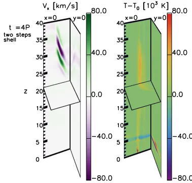
The boundary shell structure we have investigated so far is rela-tively simple, where the density smoothly increases towards the interior region and the gradient of the Alfvén speed peaks near the centre of the boundary shell. In order to address how the location of the heating depends on the structure of the bound-ary shell, we devised a different simulation where we changed the structure of the boundary into a profile with two peaks in the gradient of the Alfvén speed (Fig. 14). In this simulation the boundary shell extends from b=0.25 to a=1 (l =0.75), and the density increases in two steps similar to Eq. 1, each extend-ing for half of the boundary shell. The density profile is given by
ρ=0.5
" ρ ρe,
ρ2+ρi 2 ,a,
a+b
2
!
+ρ ρ2+ρi 2 , ρi,
a+b
2 ,b
!# .
(13)
This density profile prescribes a boundary shell of width 0.75
Mm where the density in the interior and exterior region are the
same as in the simulation with l=0.75. The two gradients of the Alfvén speed peaks are smaller and larger than the equivalent profile for the simulation with a smooth boundary shell.
Fig. 14. Density (blue lines) and gradient of Alfvén speed (red lines) across the cylinder for the simulation with a smooth boundary shell (dashed lines) and the simulation with a two-step boundary shell (con-tinuous lines).
Fig. 15. 3D cuts as in Fig. 4 of vx in the left panel and temperature
difference, (T (t)−T (0)), right panel, at t=4 P for the simulation with l=0.75 and a two-step boundary shell.
Figure 15 shows the evolution of the system at t=4 P equiv-alent to Fig. 10, and the mode-coupling and temperature increase patterns do not show great differences with respect to the sim-ulation with a smooth boundary profile. We only find that the
[image:9.612.334.523.239.419.2]vxphase-mixing pattern becomes slightly more structured with a variable width and that the temperature increases at two different locations on the boundary shell, where the temperature increase is more signficant at the more external peak.
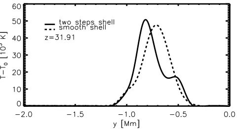
Figure 16 shows the temperature increase on the plane x=0 at z = 31.91 Mm at t = 5 P for the two simulations with a boundary shell l = 0.75 Mm. We find that the temperature in-crease follows the structure of the boundary shell, with as many temperature peaks as the gradient of the Alfvén speed peaks. The peaks are also located in the same positions as the peaks of the gradient of the Alfvén speed, and the temperature increase is proportional to the intensity of the Alfvén speed gradient.
[image:9.612.37.292.611.646.2]Fig. 16. Temperature difference, (T (t)−T (0)), cut across the cylinder on the x=0 plane at z=31.91 Mm for the simulations with l=0.75 with the smooth boundary shell (dashed line) and the two-step boundary shell (continuous line).
Fig. 17. Thermal energy difference between t and t=0 in the boundary shell as a function of time for the simulation with l=0.75 and a smooth boundary shell (dashed line) and a two-step boundary shell (continuous line).
4.3. Continuous driver
To conclude our investigation, we analysed the evolution of the system when a continuous driver (instead of a single pulse) is used to perturb the system. This is a step towards a configuration where the footpoints are continuously displaced by photospheric motion. In this simulation we used all the parameters outlined in Sect. 2, with the only difference that we did not switch offthe driver after one pulse, but let it continue.
Figure 18 shows the evolution of the system after t=6 P and
t=12 P. The vxpattern shown on the plane x=0 indicates that the phase-mixing occurs in a similar way for each consecutive period of the driver as the same pattern as is visible in Fig. 4 repeats. However, as each wave train encounters conditions that increasingly depart from the initial condition, the shape of the phase-mixing pattern becomes less regular and has more internal structuring. The temperature increase pattern shows significant differences with respect to our previous simulation, as the plasma reaches higher temperatures and the heated region broadens in time.
Figure 19 shows the temperature increase evolution of a sin-gle plasma element located at the steepest Alfvén speed location on the x =0 plane at z =26.60 Mm,and the overplotted grid is spaced one period horizontally and vertically by the temper-ature increase after one pulse. The tempertemper-ature increase starts
Fig. 18. 3D cuts as in Fig. 4 of vxin the left column and temperature
difference, (T (t)−T (0)), right column, at t=6 P (upper row) and t= 12 P (lower row) for the simulation with continuous driver.
after t = 3 P, and it increases mostly linearly until t = 7 P, when four pulses have crossed the plasma element. After t =7
P, the temperature increase is no longer linear in time, and each
pulse contributes with an increasingly smaller temperature rise. At t=12 P,the temperature increase slightly exceeds∼5×10⁵
K.
Similar conclusions can be drawn from the evolution of the energy in the boundary shell (Fig. 20), where we find that the thermal energy steadily increases until t = 11 P. After t = 2
P, the thermal energy increases at the expense of the wave
en-ergy that enters the boundary shell. However, the wave enen-ergy remains constant after t = 5 P, when the entire z-extension of the domain is filled by the wave propagation. After t=11 P, the thermal energy becomes saturated.
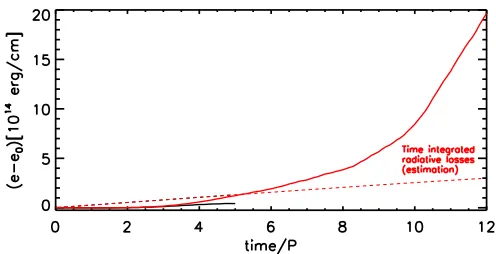
Figure 21 compares the thermal energy increase in the boundary shell at x=0 with an estimate of the radiative losses (as in Fig. 9). In this simulation the thermal energy deposition largely overcomes the radiative losses because energy is contin-uously injected into the system. It also should be noted that the increase in thermal energy is not linear, and each pulse deposits an increasingly higher amount of thermal energy because the de-position of energy drifts to lower and higher z coordinates after the shells initially involved saturate.
[image:10.612.39.294.203.367.2]Fig. 19. Temperature difference evolution of the point on the x = 0 plane at the location of the maximum gradient of the Alfvén speed at z= 26.60 Mm for the simulation with continuous driver (black continuous line), compared to the same temperature evolution for the simulation with single pulse (red line). The overplotted grid is horizontally spaced by 1 P and vertically spaced by the final temperature increase in the single-pulse simulation. The blue straight line would be the temperature evolution if the same initial temperature increase is gained at each pulse.
Fig. 20. Difference in energy in the boundary shell between time t and t=0 for the simulations with a continuous driver as a function of time: wave energy (blue line) and thermal energy (red line).
[image:11.612.309.554.12.139.2].
[image:11.612.44.288.274.438.2]Fig. 21. Thermal energy difference as a function of time integrated in the entire x=0 plane for the simulation with a continuous driver (red line) and for the simulation with a single pulse (black line). The red dashed line is an estimate of the radiative losses in the same region.
Fig. 22. Maps on the plane z=30 Mm of the temperature difference, (T (t)−T (0)) (left column), and vx(right column) at t=6 P (upper row)
and t=12 P (lower row) for the simulation with a continuous driver.
of vxand the temperature difference (T −T0) on a cross section placed at z = 30 Mm at t = 6 P and t =12 P. The cross sec-tions show regular patterns at t =6 P, when that cross section has been reached by only one pulse. The velocity patterns are concentric around the centre, and negative and positive velocity regions alternate. The temperature increase is contained within an annular arc region of the boundary shell. Once more, pulses reach this location, the patterns of vxand T −T0become more irregular, and smaller-scale structures appear. The temperature increase extends to higher radial distances from the centre of the cylinder and is no longer an annular arc. The velocity pattern also becomes irregular and involves more external shells from the centre of the cylinder. These structures develop when the system loses the initial symmetry about the x = 0 plane, and analysis of the involved forces suggests that the loss of symme-try originates from the oscillations of the magnetic field induced by the driver. This evolution is comparable with the develop-ment of Kelvin-Helmholtz instabilities reported in Terradas et al. (2008), Antolin et al. (2015), and Magyar & Van Doorsselaere (2016), with the difference that in our model the conditions for a development of the instability are built through the passage of several propagating waves, while in these studies the instability is triggered by standing oscillations. It has been shown that the development of Kelvin-Helmholtz instabilities amplifies the ef-fect of resonant absorption (or phase-mixing) of Alfvén waves on plasma heating by developing smaller-scale structures at the boundary shell where wave energy is more favourably converted into heating (Browning & Priest 1984). The present simulation shows comparable dynamics, as the thermal energy deposition in the boundary shell significantly accelerates after t = 9 P, when the first Kelvin-Helmholtz instability-like structures ap-pear. However, the high resistivity we have adopted prohibits the development of visible small-scale vortices.
One consequences of the expansion of the region involved in the temperature increase is that the heating is not bounded to the initial boundary shell, but extends in time to regions initially outside of the boundary shell. Figure 23 shows the temperature increase on the x = 0 plane at z = 26.60 Mm from t = 0 to
[image:11.612.43.291.506.633.2]Fig. 23. Temperature difference, (T (t)−T (0)), cut across the cylinder on the x=0 plane at z=26.60 Mm from t=0 to t=12 P with 1 P cadence from the thinnest to the thickest line. The red vertical dashed lines mark the borders of the boundary shell.
5. Discussion and conclusions
We have developed a simple model of a magnetised cylinder that is perturbed at one of its footpoints by a transverse displacement. The configuration we have adopted leads to the phase-mixing of propagating Alfvén waves in the loop shell region, and we focused our analysis on the heating that follows. The aim of this modelling effort is to investigate the contribution of phase-mixing of Alfvén waves to the coronal heating problem.
In many respects, our model is a simplification of a coronal loop structure, and it does not address more complex features of these magnetic structures. Certainly, our modelling starts from a condition where the coronal loop is already in place and with a temperature above the chromospheric and photospheric temper-atures. Therefore, the key to interpret our results is whether such a mechanism can at least maintain the loop structure against the radiative losses.
Although our study is not conclusive on the matter, it sheds light on some relevant aspects of the contribution from phase-mixing to coronal heating, and it helps identify some points where this model is in disagreement with observations.
First of all, our numerical experiments show that phase-mixing is a plausible mechanism in the corona, where we have used plasma and magnetic field parameters that are in the ob-served or measured range. We also showed that a time-limited oscillation propagating from the footpoint leads to a time-limited energy deposition that increases the plasma temperature by a certain amount. This process is in line with the impulsive man-ner in which coronal heating is observed to work (Warren et al. 2011; Reale 2010). Finally, we showed that the energy deposi-tion is comparable with the radiative losses, thus keeping phase-mixing as a candidate to maintain the high temperature of the so-lar corona. Given the physics and geometry of the soso-lar corona, where magnetic field structures act as vertical wave guides and observed horizontal motions at the base of the corona perturb these magnetic structures out of equilibrium, inevitably lead-ing to the upward propagation of Alfvénic waves, phase-mixlead-ing has to occur. The unanswered question is whether this is just a marginal process in the solar corona or whether it dominates the temperature evolution.
Here, major concerns are still challenging phase-mixing as a mechanism to justify coronal heating on a larger scale, and here we list some. Fist of all, the model can match the radiative loss estimation only with the adoption of a very high magnetic re-sistivity. In our simulations we used a resistivity 109times the value predicted by the classical theory (at a 2 MK temperature),
and such an amplification of the resistivity is not only essential to overcome the numerical resistivity (inherent to any MHD code), but more importantly, also to achieve a significant increase in the plasma temperature in the model. Similarly, we had to adopt a relatively large amplitude driver in order to stimulate an appre-ciable deposition of thermal energy in the model. Velocities of the order of 10 km/s are typically measured as motions of coro-nal structures, while in our case the peak velocity is higher than 100 km/s. Our velocity is also much higher than the one used in Pascoe et al. (2010), and at about 10% of the Alfvén speed, our system probably evolves in a weakly non-linear regime. More-over, the measured power spectrum of the oscillations of the solar corona peaks at 5 minutes because of the forcing photo-spheric oscillations. The period of our driver is instead at 6 sec-onds, which may not be a significant frequency of the coronal power spectrum. This is especially relevant because longer oscil-lation periods would probably lead to slower heating timescales in this model. Finally, our model has certainly led to the heating of the boundary shell, but does not address how the centre of the loop would obtain a significant amount of thermal energy to sus-tain the loop structure against radiative cooling. This is a concern intrinsic to the phase-mixing process, which concentrates wave energy only on the boundary shell (Cargill et al. 2016). Even the single case we addressed, in which the temperature increase eventually involved regions beyond the boundary shell, it needs several oscillations to set in. The question remains open whether this extension needs to be triggered earlier in order to balance radiative losses, particularly in the core of the loop.
are also a component of the spectrum and that a realistic wave packet that is more energy rich would provide the system with more energy than what we have modelled with a monochromatic pulse.
Our partial conclusion is that phase-mixing does not seem to be a viable mechanism to explain the large-scale heating of the solar corona, even though it is likely that some energy de-position takes place through this mechanism. At the same time, further analysis is needed to validate the present results and to complete the investigation. To begin with, we will run a compa-rable analysis over longer timescales and with a different class of drivers, also including the effects of radiative losses and vari-ous types of background heating in the energy balance, in order to more conclusively address whether phase-mixing can sustain the thermal structure of a coronal loop.
Acknowledgements. This research has received funding from the European
Research Council (ERC) under the European Union’s Horizon 2020 re-search and innovation programme (grant agreement No 647214) and from the UK Science and Technology Facilities Council. This work used the DiRAC Data Centric system at Durham University, operated by the Insti-tute for Computational Cosmology on behalf of the STFC DiRAC HPC Fa-cility (www.dirac.ac.uk. This equipment was funded by a BIS National E-infrastructure capital grant ST/K00042X/1, STFC capital grant ST/K00087X/1, DiRAC Operations grant ST/K003267/1 and Durham University. DiRAC is part of the National E-Infrastructure. We acknowledge the use of the open source (gi-torious.org/amrvac) MPI-AMRVAC software, relying on coding efforts from C. Xia, O. Porth, R. Keppens.
References
Antolin, P., Okamoto, T. J., De Pontieu, B., et al. 2015, ApJ, 809, 72
Arregui, I. 2015, Philosophical Transactions of the Royal Society of London Series A, 373, 20140261
Browning, P. K. & Priest, E. R. 1984, A&A, 131, 283 Cargill, P. J., De Moortel, I., & Kiddie, G. 2016, ApJ, 823, 31
De Moortel, I. & Browning, P. 2015, Philosophical Transactions of the Royal Society of London Series A, 373, 20140269
De Moortel, I. & Nakariakov, V. M. 2012, Philosophical Transactions of the Royal Society of London Series A, 370, 3193
De Moortel, I. & Pascoe, D. J. 2012, ApJ, 746, 31
Goddard, C. R., Nisticò, G., Nakariakov, V. M., & Zimovets, I. V. 2016, A&A, 585, A137
Hahn, M., Landi, E., & Savin, D. W. 2012, ApJ, 753, 36 Heyvaerts, J. & Priest, E. R. 1983, A&A, 117, 220
Jess, D. B., Mathioudakis, M., Erdélyi, R., et al. 2009, Science, 323, 1582 López Ariste, A., Luna, M., Arregui, I., Khomenko, E., & Collados, M. 2015,
A&A, 579, A127
Magyar, N. & Van Doorsselaere, T. 2016, A&A, 595, A81
McIntosh, S. W., de Pontieu, B., Carlsson, M., et al. 2011, Nature, 475, 477 Morton, R. J. & McLaughlin, J. A. 2013, A&A, 553, L10
Morton, R. J., Verth, G., Hillier, A., & Erdélyi, R. 2014, ApJ, 784, 29
Nakariakov, V. M., Ofman, L., Deluca, E. E., Roberts, B., & Davila, J. M. 1999, Science, 285, 862
Okamoto, T. J., Antolin, P., De Pontieu, B., et al. 2015, ApJ, 809, 71
Pascoe, D. J., Goddard, C. R., Nisticò, G., Anfinogentov, S., & Nakariakov, V. M. 2016, A&A, 589, A136
Pascoe, D. J., Hood, A. W., de Moortel, I., & Wright, A. N. 2012, A&A, 539, A37
Pascoe, D. J., Hood, A. W., De Moortel, I., & Wright, A. N. 2013, A&A, 551, A40
Pascoe, D. J., Wright, A. N., & De Moortel, I. 2010, ApJ, 711, 990 Pascoe, D. J., Wright, A. N., & De Moortel, I. 2011, ApJ, 731, 73 Poedts, S. & Boynton, G. C. 1996, A&A, 306, 610
Porth, O., Xia, C., Hendrix, T., Moschou, S. P., & Keppens, R. 2014, ApJS, 214, 4
Reale, F. 2010, Living Reviews in Solar Physics, 7, 5
Soler, R., Terradas, J., Oliver, R., & Ballester, J. L. 2016, A&A, 592, A28 Spitzer, L. 1962, Physics of Fully Ionized Gases (Physics of Fully Ionized Gases,
New York: Interscience (2nd edition), 1962)
Terradas, J., Andries, J., Goossens, M., et al. 2008, ApJ, 687, L115
Threlfall, J., De Moortel, I., McIntosh, S. W., & Bethge, C. 2013, A&A, 556, A124