A greedy heuristic for workforce scheduling and routing with time dependent activities constraints

J. Arturo Castillo-Salazar, Dario Landa-Silva and Rong Qu

Automated Scheduling, Optimisation and Planning (ASAP) Research Group, School of Computer Science, University of Nottingham, Jubilee Campus, Wollaton Road, Nottingham, NG8 1BB, U.K.

{psxjaca, dario.landasilva, rong.qu}@nottingham.ac.uk

Keywords: Employee Scheduling, Workforce Optimization, Personnel Routing, Greedy Heuristic, Benchmark Data, Connected Activities Constraints.

Abstract: We present a greedy heuristic (GHI) designed to tackle five time-dependent activities constraints (synchroni-sation, overlap, minimum difference, maximum difference and minimum-maximum difference) on workforce scheduling and routing problems. These types of constraints are important because they allow the modelling of situations in which activities relate to each other time-wise, e.g. synchronising two technicians to complete a job. These constraints often make the scheduling and routing of employees more difficult. GHI is tested on set of benchmark instances from different workforce scheduling and routing problems (WSRPs). We compare the results obtained by GHI against the results from a mathematical programming solver. The comparison seeks to determine which solution method achieves more best solutions across all instances. Two parameters of GHI are discussed, the sorting of employees and the sorting of visits. We conclude that using the solver is adequate for instances with less than 100 visits but for larger instances GHI obtains better results in less time.

1

INTRODUCTION

The workforce scheduling and routing problem (WSRP) refers to the assignation of a diverse skilled workforce to a series of visits at different locations. Each visit requires an activity completion before trav-elling to the next visit. Activities require different skills and might need more than one employee. Other constraints which relate activities to each other, i.e. connected activities constraints, are also present in WSRP (Castillo-Salazar et al., 2014). Particularly, in this paper we focus on those connected activi-ties constraints that are time-dependent (synchronisa-tion, overlap, minimum difference, maximum differ-ence and minimum-maximum differdiffer-ence). These type of connected activities constraints are also known in the literature as temporal dependencies (Rasmussen et al., 2012) or interdependant services (Mankowska et al., 2014). For applications and solution meth-ods of WSRP in sectors such as home health-care (Akjiratikarl et al., 2007; Kergosien et al., 2009), security provision (Misir et al., 2011; Chuin Lau and Gunawan, 2012), retail and maintenance services (Cordeau et al., 2010; G¨unther and Nissen, 2012), etc. we refer the reader to the survey by Castillo-Salazar et al. (2012) . In such sectors, daily employee

schedul-ing and routschedul-ing is necessary to complete a diverse set of activities across several client locations. In what follows, we use connected activities constraintsand time-dependent constraints indistinctly. These con-straints allow to model situations in which two activ-ities need to start at the same time, e.g. two techni-cians to calibrate a fiber optic segment. Also, when one activity needs to start after the completion of an-other one, e.g. a care worker to help ironing only after completing the washing. The related activities do not have to be performed by the same employee.

con-straints. They used an adapted version of the mixed integer linear model by Rasmussen et al. (2012) . The model was solved by a state of the art solver in order to provide benchmark results. Nevertheless, no other solution method was explored. The benchmark presents a series of daily real-based problems. The authors clarify the need to obtain good enough solu-tions within a reasonable time. For real-world based instances, daily problems need to be solved during the night before the planning day if not faster. Solving WSRP as close as possible to the start of the plan-ning horizon helps to include all updated availabil-ity of employees. Nevertheless, often changes are required due to unexpected absences or urgent prior-ity services. In their experiments, Castillo-Salazar et al. (2014b) used two hours as maximum computa-tional time. It has been reported that medium to large WSRP instances cannot be solved using a mathemat-ical solver within 10 hours (Mankowska et al., 2014) and for some small instances solvers could require 67 hours to prove optimality (Castillo-Salazar et al., 2014). Our objective when developing the greedy heuristic is to obtain at least the same quality of sults as the solver (measured by the gap to the re-ported lower bound) in the benchmark data set but faster, as this would help to incorporate unexpected changes near the start of the planning horizon.

A greedy heuristic is a procedure based on con-secutive decisions that at every step, if possible, leads to a better result. Greedy heuristics rely in some in-formation about the domain of the problem and of-ten obtain good feasible results in short time. Al-though, there are greedy heuristics that have tackled workforce scheduling and routing problems (Xu and Chiu, 2001; Mankowska et al., 2014), to the best of our knowledge none can support time windows on activities that are also related to other activities by any of the 5 types of time-dependent constraints. The main contribution of this work is tackling activities that have any of the 5 time-dependent constraints.

There are four more sections in this paper. Section 2 explains the MILP model of the WSRP. Section 3 presents the proposed greedy heuristic. Section 4 de-scribes the experiments settings. Section 5 presents our results. Finally, section 6 concludes the paper.

2

MIP MODEL FOR WSRP

The MILP model used as a reference to compare the greedy heuristic can be found in (Castillo-Salazar et al., 2014). Here we provide an overview of it.

Crepresents the set of visit locations. 0k_andnk

re-fer to the starting and ending locations for employee

k. K is the set of employees. Nk=C∪ {0k,nk}is the set of available locations for employeek. Activ-ityistarting time window is given by two valuesαi

(earliest start time) and βi (latest start time). Binary

variableρk_i is set to 1 if employeekcan perform ac-tivityibased on skill requirement, and 0 if not. Activ-ities can be left unassigned when there is not enough employees to perform all of them. Binary variableyi

is set to 1 if activityiis left unassigned and 0 other-wise. The duration of activityi plus the travel time from activity locationito activity location jfor em-ployeekis given bysk_{i j}. The starting time of activity iby employeekist_ik. Employeekstarts his working time atα_nk and must finish byβ_nk. Time-dependent

constraints are indicated by a set of pairs of activities P. For every pair of activitiesiandj, a constant value pi jis given depending on the type of time-dependent

constraint (Rasmussen et al., 2012, pg. 601). Finally, binary variablesxk_{i j}are set to 1 if employeekmoves to activity location jafter performing activityi. Minimise:

ω1

_∑

k∈Ki∈N

∑

∑

Ck_{i j}xk_{i j}+ω2

_∑

∑

∑

δk_ixk_{i j}+ω3

_∑

γiyi

(1) Subject to:

∑

∑

xk_{i j}+yi=1 ∀i∈C, (2)

∑

xk_{i j}≤ρk_i ∀k∈K, ∀i∈C, (3)

∑

xk

0k_,j=1 ∀k∈K, (4)

∑

xk

i,nk=1 ∀k∈K, (5)

∑

xk_ih−

_∑

xk_{h j}=0 ∀k∈K, ∀h∈C, (6)

αi

_∑

xk_{i j}≤t_ik∀k∈K,∀i∈C∪ {0k}, (7)

t_ik≤βi

_∑

xk_{i j}∀k∈K,∀i∈C∪ {0k}, (8)

α_nk≤tk

nk≤βnk∀k∈K, (9)

t_ik+sk_{i j}x_{i j}k ≤tk_j+βi(1−xki j)∀k∈K,∀i,j∈Nk,(10)

αiyi+

_∑

t_ik+pi j≤

_∑

tk_j+βjyj∀(i,j)∈P,(11)

x_{i j}k ∈ {0,1} ∀k∈K,∀i,j∈Nk,(12)

t_ik∈R+∀k∈K,∀i∈Nk,(13)

yi∈ {0,1} ∀i∈C.(14)

consid-ers employees preferences with regards to activities. Employeekpreference to perform activityiis given by the term (δk_i). Finally, the priority of the

activ-ities is also consider in the objective function since some locations might not be visited and therefore its activity left unassigned. Activityipriority is given by

γi. Every component of the objective function has a

weight associated. The weights (ω1,ω2,ω3) are set as

in (Rasmussen et al., 2012).

Constraints are as follows: visits are either per-formed or left unassigned (2). Activities can only be assigned to employees able to perform them (3). All employees must start from the initial location (4) and return to their own final location (5). Constraint (6) ensures that once employeekvisits activity location h, he leaves it, i.e. it maintains flow conservation. Time windows of visits must be satisfied (7, 8). Vis-its should be performed during the employees starting and ending times (9). Constraint (10) ensures travel-ling times are respected by the start of activities. Con-nected activities constraints (11) exist among related activities. Decision variablesxk_{i j}are set to 1 when em-ployeektravels from locationito jand 0 otherwise (12). Scheduling variables are positive integers (13). Finally, if an activityiis not performed the binary de-cision variablesyiis set to 1 and 0 otherwise (14).

3

GREEDY HEURISTIC (GHI)

The data structure that holds the solution at any time is presented in Figure 1. The main list is defined by the number of employees plus one additional node for unassigned visits. Within each node there is a list of visits which the employee has been assigned to. The list of visits is maintained in ascending order accord-ing to time. Rectangles represent activity duration, traveling time, and idle time. The last rectangle of each list of activities represents the traveling time to the ending location of the employees. Activities in the bottom node (Unassigned) have no particular order. The proposed constructive heuristic GHI works as follows (Algorithm 1). It starts by creating a copy visitList with all visits, creating the solution struc-ture described above and sortingvisitList according tolistCriterion (section 3.1.1). In each iteration of the assignation cycle (lines 5 to 13), GHI sorts the solution structuresol according tosolCiterion (sec-tion 3.1.2) and processes the next visit vfrom Vis-itList. For processing, visitvis passed to the PRO

-CESS function which returns the list of related vis-itslrv(step 8). Then, each visit v2 (if any) related tovthrough a connected activity constraint, is pro-cessed by the PROCESSDEP function which

consid-Figure 1: Solution structure for WSRP.

ers the constraint and maintains feasibility (lines 9 to 13). Processingvand its dependent visitsv2 means that they are removed from thevisitListand a new it-eration starts. This assignation cycle continues until no visits are left invisitList.

Algorithm 1:GHI: SOLVE.

1: procedureSOLVE

2: visitList←copy ofvisits(V)

3: sol←CREATESOLUTIONSTRUCTURE 4: SORT(visitList, listCriterion)

5: whilevisitList is not emptydo

6: SORT(sol, solCriterion)

7: v←visitList.remove(0)

8: lrv←PROCESS(v) 9: iflrv.size>0then

10: whilelrv is not emptydo

11: v2←lrv.get(0)

12: lrv←PROCESSDEP(v,v2,lrv)

13: visitList.remove(v2)

We tackle activities with time-dependent con-straints by creating different functions for the inde-pendent and the deinde-pendent activities within such con-straints. We seek to assign the independent activity first as this provides the starting time upon which the dependent activities adhere to. Functions PROCESS

for independent activities (Algorithm 2) and PRO

as result (steps 14 & 15). PROCESSDEPworks simi-larly but also considers any time-dependent constraint involvingv2 (step 3). PROCESSDEP requires thatv is assigned to use its start time to enforce the time-dependent constraint in all its related visitsv2.

Algorithm 2:GHI: PROCESS.

1: procedurePROCESS(v)

2: can←ALLOCPOSSIBLEANY(v,sol) 3: SORT(can)

4: ifcan is not emptythen

5: ca←can.remove(0)

6: INCLUDE(c,sol)

7: i←v.required

8: for i>1do

9: ifcan is not emptythen

10: ca←can.remove(0)

11: INCLUDE(ca,sol)

12: else

13: UNALLOCATE(v,sol) 14: lrv←GETRELATED(v)

15: returnlrv

Algorithm 3:GHI: PROCESSDEP.

1: procedurePROCESSDEP(v,v2,lrv)

2: can←ALLOCPOSSIBLEANY(v2,sol) 3: CONSIDERRC(v,v2,can)

4: ifcan is not emptythen 5: SORT(can)

6: ca←can.remove(0)

7: INCLUDE(ca,sol)

8: i←v.required

9: for i>1do

10: ifcan is not emptythen

11: ca←can.remove(0)

12: INCLUDE(ca,sol)

13: else

14: UNALLOCATE(v,sol)

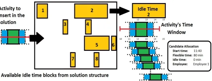
Within PROCESSand PROCESSDEP, the ALLOC -POSSIBLEANY function looks for idle times in an employee daily schedule. The INCLUDEfunction as-signs the candidate structure with possible allocations to the solution structure. The UNALLOCATEfunction unassigns a visit from its current employee schedule and leaves it in the unassigned node. GETRELATED

identifies other activities that are time-dependent tov via a connected activity constraint.

ALLOCPOSSIBLEANY(Algorithm 4) is the func-tion that searches the solufunc-tion structure to find idle time so that new activities can be assigned. It returns a collection of candidate allocations. It iterates the

Algorithm 4:GHI: ALLOCPOSSIBLEANY.

1: functionALLOCPOSSIBLEANY(v,sol)

2: forn←sol.nodesdo

3: emp←n.emp

4: if¬PERFORM(emp,v)then

5: next

6: ifn.sch is emptythen

7: w←LASTAVWINDOW(n.sch) 8: ca←ENOUGH(w,v.win,emp) 9: ifca is not nilthen

10: can.add(ca)

11: else

12: forw←1,n.schdo

13: ca←ENOUGH(w,v.win,emp) 14: ifca is not nilthen

15: can.add(ca)

16: w←LASTAVWINDOW(n.sch) 17: ca←ENOUGH(w,v,emp) 18: ifca is not nilthen 19: can.add(ca)

whole structure looking for idle times where the visit (v) can be inserted, it considers the travel time to get to the visit and the difference in travel time from the visit to the following destination (ENOUGH). It avoids exploring nodes representing employees that cannot perform the activity of the visit (PERFORM). LAS

-TAVWINDOW returns the last idle block in an em-ployee schedule. The last idle block is defined as the time between the last activity completion and the em-ployee’s shift ending. This is a special case because it needs to consider the travel time to the ending loca-tion of the employee.

A candidate allocation structure represents several possible employee-activity assignations. It is defined by a starting time, a flexible component, idle time and a worker reference. The starting time provides the first possible start time in which an activity can start, the flexible component provides a time length which that start time can be delayed and still fit in the idle block. Idle time represents the time left before the starting time. Figure 2 shows how a candidate alloca-tion structure is formed. The line indicates the activ-ity’s time window, the series of dark blocks represent the number of possibilities that the activity could fit in the idle space number 2.

re-Figure 2: Represents how the AllocPossibleAny function considers idle time blocks and creates candidate allocations.

Figure 3: Examples of how the heuristics consider each of the connected activities constraints.

pair mechanism is to leave all activities with time-dependent constraints unassigned, because if a visit is left unassigned then any constraints that it relates to are disabled by the logic of the model. But, we now aim to process those constraint early in the cre-ation of the solution and keep them satisfied because leaving visits unassigned comes at a high cost. There-fore, GHI includes a preventive step which verifies if the current visit is associated with another visit (via a connected activities constraint) and if so, it tries to al-locate the related visit in a suitable manner after con-sidering the starting time of the first visit to comply with the constraint. Such procedure is described in Figure 3 dealing with each of the 5 connected activ-ities constraints (overlapping, synchronisation, mini-mum, maximum and min-max time difference). Fig-ure 3 shows an example for each type where activ-ities A and B are related by each of the connected activities constraint types. In the figure, the dark rect-angle is the activity duration, the lighter rectrect-angle is the flexible time (the activity can move forward and still comply with other time constraints), the dotted line inside the dark rectangle is the latest start time for the activity. Every example in the figure considers two cases, first (left one) both activities A and B com-ply with the time-dependent constraint, second (right

one) delays the start of A or B so we can comply to a constraint that otherwise would not be enforced. For example, in the maximum difference sub-figure, the right case shows B starting within the maximum time allowed after the A starting. The left shows that A starting as originally makes B starting after the max-imum allowed period. By delaying A (arrow shifting A to the right), activity B now enters into the max-imum allowed zone, hence satisfying the constraint. Notice, that B could not be started earlier because it was already at its earliest starting time.

3.1

Parameters of the Greedy Heuristic

GHI has two parameters that need to be set, ones is listCriterion, the sorting of the list of activities dur-ing initialisation and the other one issolCriterion, the solution structure sorting after each iteration.

3.1.1 ParameterlistCriterionValues

Durationsorts visits in descending order based on the

duration of the activity (v.dur).

Maximum Finish Timesorts visits in ascending

Maximum Start Timesorts visits in ascending order based on the maximum time the visit can start given its time window. The sorting parameter isv.lst.

Minimum Finish Timesorts visits in ascending

or-der based on the minimum time the visit can finish given its time window. The sorting parameter isv.eet.

Minimum Start Timesorts visits in ascending order

based on the minimum time the visit can start given its time window. The sorting parameter isv.est.

Number of Employeessorts visits in descending

or-der based on the number of employees required. The parameter for sorting isv.req.

Density sorts visits in descending order based on

the density factor. The density factor is obtained by adding the number of employees required plus the number of connected activities constraints that the visit is involved in. This aims to process activities that are more constrained first and leave the simpler ones at the end. The number of employees in the team is modelled using synchronisation constraints.

3.1.2 ParametersolCriterionvalues

Remaining Timesorts the solution list in descending

order based on the time available left for every em-ployee. The time available is calculated from the last visit until the end of the employees shift minus the time needed for the trip to the ending location. In all the instances, shift starting and finishing times coin-cide with the beginning and end of the time horizon. It aims to reduce the number of employees, since it avoids using a new employee unless the available time of the previous ones are full or no other allocation is possible. If the sorting is in ascending manner, visits will be balanced across all possible employees with the right skills.

Solution Sizeorders the solution structure main list

in ascending order based on the number of visits that employees have. When two nodes have the same number of visits, the tie-break criterion is the longest remaining time explained above.

4

EXPERIMENTS

The aim of the experiments is to evaluate the quality of the solutions obtained by GHI when compared to the solver. The comparison seeks to determine which solution method achieves more best solutions across all instances.

In this study we used the benchmark data set from Castillo-Salazar et al. (2014b). The data set is an adaptation of different WSRP from the literature. We used 4 groups of instances Sec, Sol, Mov and HHC.

Sec is based on security guards patrolling different buildings (Misir et al., 2011). Sol is based on adap-tations to the Solomon data set. Three different ver-sion of each instance are used 25, 50 and 100 vis-its (Solomon, 1987). Mov originates from a multi-objective VRPTW study which controlled variability of time window sizes (Castro-Gutierrez et al., 2011). HHC is a home health care data set. It includes a good level of skills, preferences on employees and patients (Rasmussen et al., 2012). The total number of in-stances used is 374. The original benchmark has 375 instances, the instance that is not being used belong to a single-instance group of technicians on field for which the benchmark does not provides results.

All instances are solved first using a mathematical solver. A time limit of 2 hours is set for the solver and we keep the solution found after this. The solver achieves optimal solutions for 33 instances. There are 37 instances in which no solution was found by the solver within the time limit. All instances are solved also by GHI (coded in Java). As part of our experi-ments we want to find which combination of values for listCriterion(7 possible values) andsolCriterion (2 possible values) obtains the best results. Therefore, GHI is executed for all 374 instances for the 14 com-binations of parameters. We use all comcom-binations to identify the best values for the two parameters.

5

RESULTS

Out of the 374 instances, the solver obtained better results for 187. GHI also obtained 187 best feasible solutions. For none of the instances solver and heuris-tic produced the same result.

In Figure 4 the results are segmented for each of the 4 data sets. GHI has better results than the solver

inSec,HHCandMov. In groupSolthe solver

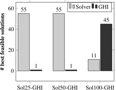
out-performs the heuristic. In order to investigate this fur-ther we analyse the three subgroups within the Sol group. The subgroups are those with 25, 50 and 100 visits. Figure 5 shows the subgroups segmented re-sults. The solver is better in subgroups with 25 and 50 visits. But for instances of 100 visits GHI out-performs the solver. GHI obtained the same number of best feasible result as the solver. However, overall GHI is significantly faster spending less than 1 second in each instance.

5.1

Evaluating the Quality of Results

Sec-GHI Sol-GHI HHC-GHI Mov-GHI 0

50 100

61

121

0 5

119

47

11 10

#

best

feasible

solutions

Solver GHI

Figure 4: Results GHI when compared to the solver. The graphs show the number of best feasible solutions obtained by each method. The results are segmented according to the data set group the belong (Sec, Sol, HHC and MOV).

Sol25-GHI Sol50-GHI Sol100-GHI 0

20 40

60 _{55 55}

11

1 1

45

#

best

feasible

solutions

Solver GHI

Figure 5: Solomon 25, 50 and 100 visitsSolsub-groups re-sults of GHI (in red) when compared to the solver (in blue).

instances in 4 groups depending on the results ob-tained. The first group are instances for which the solver obtained optimal solutions, the gap from the GHI to the optimal is reported. The second group are instances for which the solver obtained better fea-sible solutions but not optimal, the gap between the GHI and the best feasible solution by the solver is reported. The third group are instances where GHI is better than the solver, the gap between the solver and GHI is reported. Finally, the fourth group are instances where no solutions were obtained by the solver within the time limit, no gap is provided for this group. The gap calculation for groups 1 and 2 is (GHI−Solver)/ABS(Solver) and for group 3 is(Solver−GHI)/ABS(GHI). The principle is the same, because it is a minimisation problem, in every group we subtract the best result(minimum) from the worst one(maximum) and normalise according to the best one(minimum). Absolute value of the

denomina-tor is necessary to avoid providing negative gaps.

Table 1: Group result type: 1 optimal, 2 solver best, 3 GHI best and, 4 only GHI available. Number of instances #, mean number of employees µemp, mean number of visits µvisits, mean time horizon durationµtHor, mean visit dura-tionµv.durand mean time window sizeµv.win.

G # µemp µvisits µtHor µv.dur µv.win

1 33 12.8 43.1 1817.3 60.3 291.7 2 154 10.3 47.0 1088.1 149.8 382.9 3 150 26.3 117.2 1311.6 284.7 422.9 4 37 66.0 171.6 1147.8 333.9 402.8

Table 1 shows some characteristics of each group. GHI found better results in groups 3 and 4, which have on average more employees, more visits, longer visits and longer time window sizes. The solver per-forms better in groups 1 and 2, but could only find optimal solutions for group 1. There is not signifi-cant difference in the average number of visits (43.1 vs 47.0) and employees (12.8 vs 10.3) between group 1 and 2. But, group 2 seems more difficult for the solver. We argue that not only the number of employ-ees and visits define how difficult a WSRP might be. Other factors like duration of visits, time to perform them (time horizon) and flexibility of time windows could also affect the degree of difficulty as shown by group 2 when compare to group 1. Group 2 has longer visits to perform in less time (time horizon) with greater flexibility of the time windows.

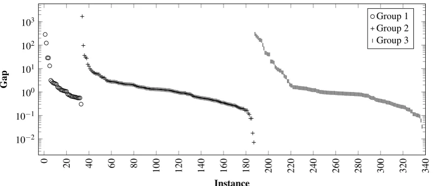
Figure 6 plots the gap result of groups 1, 2 and 3. The overall observation for group 1 (GHI vs. optimal solution), is that no gap was less then 10% and for 1/2 of the instances the gap was 77% or less. For group 2 (feasible but not optimal solutions by the solver better than GHI), the minimum gap achieved was 1% and for 1/2 of the instances the gap is less than 63% (for the other 1/2 the gap was higher). Finally, for group 3 (feasible but not optimal solutions by the solver worse than GHI), the minimum gap achieved was less than 1% but only 1/4 of the instances had a gap less than 68% (for the other 3/4 the gap was higher). THs means that GHI is a better runner-up against the solver than the opposite. For the solver to do better in group 3, the computational time needs to be increased sub-stantially. This is investigated in the next section.

5.1.1 Increasing Computational Time

ob-0

20 40 60 80 _{100 120 140 160 180 200 220 240 260 280 300 320 340} 10−2

10−1 100 101 102

103

Instance

Gap

Group 1 Group 2 Group 3

Figure 6: Gap plot for instances in Group 1-blue, Group 2-red and Group 3-black. Notice the logarithmic scale in the y-axis.

tain better results than GHI with a gap of less than 2% within the 4 hours. Therefore, even doubling the com-putational time does not really make the solver a bet-ter runner-up on the instances of group 3. The same behaviour has been reported in the literature (Castillo-Salazar et al., 2014) for this benchmark data set, after two hours the solver improvements are minimal and at a high cost (in computational time).

6

CONCLUSION

This paper presents a deterministic greedy heuristic (GHI) to tackle the workforce scheduling and rout-ing problem (WSRP). We perform computational ex-periments using a data set consisting of 374 instances from four different WSRP scenarios. The proposed heuristic needs only two parameters. One to decide the order in which activities are processed. The other one to decide the order in which employees are con-sidered for the assignation. This tailored heuristic is able to tackle time-dependent activities constraints which arise when activities are related to each other. We run experiments to compare the results obtained by GHI against the results produced by a commercial mathematical programming solver. Our experiments also seek to identify the best settings for the two pa-rameters mentioned above.

The deterministic greedy heuristic GHI generates better results for one half of Castillo-Salazar et al. (2014b) benchmark instances. Apart from the reduc-tion in the objective funcreduc-tion value, GHI runs at a marginal time (less than 1 second) compared to the two hours given to the solver. For the instances in which the solver produces better results, GHI follows closely. But for the instances in which GHI produces

better results, the solver stays far behind even after doubling the computation time. In relation to GHI’s parameter setting, we found no difference between the two values forsolutionCriterion, but forlistCriterion, time-based sorting is better. This is because the range of values provided by the time-based sorting mecha-nism facilitates a better distribution of the visits. It is left for future investigation whether combining two sorting mechanisms inlistCriterion, e.g. density with minimum start time could produce better results. The hypothesis is that density could help allocate complex visits first, such as those requiring multiple employees or involved in time-dependent activities constraints, whilst the time-based sorting could impose a better order to those activities that are less complex.

Given our results we conclude that for instances with less than 100 visits, a mathematical solver is likely to provide an optimal solution or a good fea-sible solution. As soon as the number of visits raises, the quality of the solution obtained by the solver de-creases, and in some cases no solution is found within two hours. We also demonstrated than increasing the time limit of the solver to 4 hours in those instances in which the solver is runner-up to GHI, does not help the solver to perform better than GHI. Therefore, for obtaining good-quality feasible solutions for in-stances with more than 100 visits in fast computation time, we suggest the use of GHI. Future work will consider using GHI for providing an initial solution to a meta-heuristic method such as Tabu Search.

ACKNOWLEDGEMENTS

REFERENCES

Akjiratikarl, C., Yenradee, P., and Drake, P. R. (2007). Pso-based algorithm for home care worker schedul-ing in the uk. Computers & Industrial Engineering, 53(4):559–583, doi:10.1016/j.cie.2007.06.002. Castillo-Salazar, J. A., Landa-Silva, D., and Qu, R. (2012).

A survey on workforce scheduling and routing prob-lems. In Proceedings of the 9th International Con-ference on the Practice and Theory of Automated Timetabling (PATAT 2012), pages 283–302, Son, Nor-way.

Castillo-Salazar, J. A., Landa-Silva, D., and Qu, R. (2014). Workforce scheduling and routing problems: litera-ture survey and computational study.Annals of Oper-ations Research, doi:10.1007/s10479-014-1687-2. Castro-Gutierrez, J., Landa-Silva, D., and Moreno-Perez,

J. (2011). Nature of real-world multi-objective ve-hicle routing with evolutionary algorithms. In Sys-tems, Man, and Cybernetics (SMC), 2011 IEEE In-ternational Conference on, pages 257 –264.

Chuin Lau, H. and Gunawan, A. (2012). The patrol schedul-ing problem. InProceedings of the 9th International Conference on the Practice and Theory of Automated Timetabling (PATAT 2012), pages 175–192, Son, Nor-way.

Cordeau, J.-F., Laporte, G., Pasin, F., and Ropke, S. (2010). Scheduling technicians and tasks in a telecommuni-cations company. Journal of Scheduling, 13(4):393– 409, doi:10.1007/s10951-010-0188-7.

G¨unther, M. and Nissen, V. (2012). Application of parti-cle swarm optimization to the british telecom work-force scheduling problem. InProceedings of the 9th International Conference on the Practice and Theory of Automated Timetabling (PATAT 2012), pages 242– 256, Son, Norway.

Kergosien, Y., Lente, C., and Billaut, J.-C. (2009). Home health care problem, an extended multiple travelling salesman problem. In Blazewicz, J., Drozdowski, M., Kendall, G., and McCollum, B., editors,Proceedings of the 4th Multidisciplinary International Scheduling Conference: Theory and Applications (MISTA 2009), pages 85–92.

Mankowska, D. S., Meisel, F., and Bierwirth, C. (2014). The home health care routing and scheduling prob-lem with interdependant services. Health Care Man-agement Science, 17:15–30, doi:10.1007/s10729-013-9243-1.

Misir, M., Smet, P., Verbeeck, K., and Vanden Bergue, G. (2011). Security personnel routing and rostering: a hyper-heuristic approach. InProceedings of the 3rd International Conference on Applied Operational Re-search, ICAOR11, Istanbul, Turkey, 2011, pages 193– 206.

Rasmussen, M. S., Justesen, T., Dohn, A., and Larsen, J. (2012). The home care crew scheduling problem: Preference-based visit clustering and temporal depen-dencies. European Journal of Operational Research, 219(3):598–610, doi:10.1016/j.ejor.2011.10.048. Solomon, M. M. (1987). Algorithms for the vehicle

routing and scheduling problems with time windows

constraints. Operations Research, 35(2):254–265, doi:10.1287/opre.35.2.254.