A New Parametric Estimation Method for Graph-based Clustering
Abstract
Relational clustering has received much attention from researchers in the last decade. In this paper we present a parametric method that employs a combination of both hard and soft clustering. Based on the corresponding Markov chain of an affinity matrix, we simulate a probability distribution on the states by defining a conditional probability for each subpopulation of states. This probabilistic model would enable us to use expectation maximization for parameter estimation. The effectiveness of the proposed approach is demonstrated on several real datasets against spectral clustering methods.
1 Introduction
Clustering methods based on pairwise similarity of data points have received much attention in machine learning circles and have been shown to be effective on a variety of tasks (Lin and Cohen, 2010; Macropol, et al., 2009; Ng, et al., 2001). Apart from pure relational data e.g. Biological networks (Jeong, et al., 2001), Social Networks (Kwak, et al., 2010), these methods can also be applied to none relational data them e.g. text (Ding, et al., 2001; Ng, et al., 2001), image (Shi and Malik 2000), where the edges indicate the affinity of the data points in the dataset.
Relational clustering has been addressed from different perspectives e.g. spectral learning (Ng, et al., 2001; Shi and Malik 2000), random walks (Meila and Shi 2000; Macropol, et al., 2009), trace
maximization (Bui and Jones, 1993) and
probabilistic models (Long, et al., 2007). Some works have proposed frameworks for a unified
view of different approaches. In (Meila and Shi 2000) a random walk view of the spectral clustering algorithm in (Shi and Malik 2000) was presented. By selecting an appropriate kernel, kernel k-means and spectral clustering are also proved to be equivalent (Dhillon, et al., 2004). As shown in (von Luxburg, 2007) the basic idea behind most methods are somehow optimizing the normalized cut objective function.
We propose a new perspective on relational clustering where we use the corresponding Markov chain of a similarity graph to iteratively cluster the nodes. Starting from a random distribution of nodes in groups and given the transition probabilities of the Markov chain, we use expectation maximization (EM) to estimate the membership of nodes in each group to eventually find the best partitioning.
After a brief review of the literature in section 2, we present our clustering algorithm in detail (section 3) and report experiments and evaluation (section 4).
2 Background and Related Work
Due to the wealth of literature on the subject, it’s a formidable task to give a thorough review of the research on relational clustering. Here we give a brief review of the papers that are more well-known or related to our work and refer the reader to (Chen and Ji 2010; Schaeffer 2007; von Luxburg, 2007) for more detailed surveys.
Graph clustering can be defined as finding k
disjoint clusters 1, . . ⊂ in a graph G = (V, E) where the vertices within each clusters are similar to each other and dissimilar to vertices in
Javid Ebrahimi and Mohammad Saniee Abadeh
Faculty of Electrical & Computer Engineering Tarbiat Modares University
Tehran, Iran
{j.ebrahimi,saniee}@modares.ac.ir
other clusters. Cut based measures, among others can be used to identify high quality clusters. Minimum cut of a graph is a cut (1) with the lowest value.
=
∈ , ∉
(1)
Here is the number of clusters and is the cluster. Normalized cut (2) is a better objective function that evades minimum cut's bias toward smaller clusters by incorporating total connection from each cluster to all nodes in the graph. In their seminal work Shi and Malik (2000) transformed the normalized cut to a constrained Rayleigh quotient and solved it by a standard eigenvalue system.
_ =
∈ , ∉ ,
∈
(2)
Spectral clustering makes use of the spectrum of a graph: either the eigenvalues of its affinity matrix
or its Laplacian matrix (Schaeffer 2007). For
example in (Ng, et al., 2001) the k largest
eigenvectors of normalized graph Laplacian matrix
is selected, the rows of the inverse of the resultant matrix are unit normalized and are finally clustered into k clusters using k-means. Roughly speaking, spectral clustering embeds data points in a low-dimensional subspace extracted from the similarity matrix, however this dimension reduction may ensue poor results when the approximation is not good (Lin and Cohen 2010).
Meila and Shi (2000) showed that the
corresponding stochastic matrix of an affinity matrix has the same eigenvectors as the normalized Laplacian matrix of the graph, thus spectral clustering can be interpreted as trying to find a partition of the graph such that the random walk stays long within the same cluster and seldom jumps between clusters (von Luxburg, 2007). The Markov clustering algorithm (MCL) (van Dongen 2000) is another algorithm that addresses graph clustering from a random walk point of view. MCL calculates powers of associated stochastic matrix of the network and strengthens the degree of connectivity of densely linked nodes while the sparse connections are weakened. Repeated
random walk (RRW) (Macropol, et al., 2009) addresses MCL’s sensitivity to large diameter clusters and uses random walk with restart method to calculate relevant score of connectivity between nodes in the network. Then, it repeatedly expands based on relevant scores to find clusters in which nodes are of high proximity. We should bear in mind that most random walk based algorithms have been designed primarily for biological networks where the number of clusters is unknown and some parameters e.g. desired granularity, minimum or maximum size of clusters might be needed for a meaningful interpretation of biological data. On the other hand, spectral clustering methods need to know the number of clusters beforehand but don’t need tuning parameters and are more practical.
In this paper, we adopt an approach similar to probabilistic and partitional clustering in Euclidean space, where the algorithm starts from random guesses for some parameters and iteratively clusters the data and improves the guesses. In other words instead of embedding data points in the Eigen space or powering of the stochastic matrix, we’re looking for a probabilistic model that solely employs the relation between data points.
3 Clustering Algorithm
3.1 Notation
Given a dataset D = ( ), ( ), … , a
similarity function s( ( ), ( )) is a function where
s( ( ), ( )) = s( ( ), ( )) , s ≥ 0 and s = 0 if i = j. An affinity matrix ∈ ℛ × is an
undirected weighted graph defined by =
s( ( ), ( )) . after row-normalizing the affinity
matrix, we find the stochastic matrix ∈ ℛ × of
the corresponding Markov chain (MC) with states
( ), ( ), … where ∑ = 1 .
3.2 Hard-Soft Clustering
The basic idea behind Hard-Soft clustering (HSC) is to put nodes in clusters where within cluster transitions are more probable and between cluster
transitions are minimal. HSC makes use of both
to model hard guesses could be described by a mixture of multinomial model where the parameters (probabilities), are discretized {0, 1}. We start from random hard guesses and iteratively improve them by maximizing the likelihood using
EM. Let ( ), ( ), … ( ) denote the states of
the MC and given the number of clusters, what is the maximum likelihood of hard partitioning of nodes? Having as the number of clusters and
as number of nodes is a × matrix that
shows which node belongs to which cluster i.e. one in the corresponding element and zero otherwise. The likelihood function is as follows:
ℓ( ) = ∑ ∑ ( ) ( ); ) ( );
( ) (4)
In (4), ( )~ ( ) is our latent random
variable where the mixing coefficient
gives ( ( )= ). For the soft clustering part of
HSC, we define the prior distribution ( ) ( )=
; ) as the probability of transitioning from ( )to
states marked by row vector (∑ ) . This
conditional prior distribution simulates a
probability distribution on the states in the MC because Pr ( ( )) along with the joint distribution
∏ Pr ( ( )) barely have any real world
interpretation.
The E-step is computed using the Bayes rule:
( )
∶= ( )= ( ); ) =
( ) ( )= ; ) ( ( )= ; )
∑ ( ( )| ( )= ; ) ( ( )= ; ) (5)
The M-step (6) is intractable because of the logarithm of the weighted sum of parameters.
max ( ) = ( )log(∑ ( ) ) (6)
s.t∑ = 1
However since the weights are transition
probabilities and ∑ = 1 , we can use
weighted Jensen’s inequality to find a lower bound
for ( ), get rid of logarithm of sums and convert
it to sum of logarithms.
( ) ≥
( ) = ( ) log + log − log ( )
The weighted Jensen’s inequality ( ) ≥ ( )
holds with equality if and only if for all the
with ≠ 0 are equal (Poonen 1999), which is
not applicable to our case since taking the constraint into account, all nodes would have
membership degrees to all clusters ( = ),
therefore the inequality changes to a strict inequality ( note that we have relaxed the problem
so that can take fractional values that will
eventually be discretized {0, 1}, for example
setting one for the maximum and zero for the rest), Nevertheless maximizing the lower bound still
improves previous estimates and is
computationally more efficient than maximizing
( ) itself which would require none linear
optimization. Taking the constraint into account we use Lagrange multipliers to derive the parameters.
ℒ( ) = ( ) log + log − log ( )
− ( − 1)
ℒ( ) = ( ) − = 0
= ∑ ( )
∑ ∑ ( ) (7)
To avoid bias toward larger clusters is further
row-normalized. Similarly can be calculated:
= 1 ( ) (8)
Algorithm: HSC
Input: The stochastic matrix P and the
number of clusters c
Pick an initial and .
repeat
E-step: ( )=
( ) ( )
; )
∑ ( ) ( ) ; )
M-Step: = ∑
( )
∑ ∑ ( ) ; = ∑ ( )
Row-normalize and then discretize H. until does not change
4 Experiments
4.1 Datasets
We use datasets provided in (Lin and Cohen 2010). UbmcBlog (Kale, et.al, 2007) is a connected network dataset of 404 liberal and conservative political blogs mined from blog posts. AgBlog (Adamic and Glance 2005) is a connected network dataset of 1222 liberal and conservative political blogs mined from blog home pages. 20ng* are subsets of the 20 newsgroups text dataset. 20ngA
contains 100 documents from misc.forsale and
soc.religion.christian. 20ngB adds 100 documents to each category in 20ngA. 20ngC adds 200 from
talk.politics.guns to 20ngB. 20ngD adds 200 from
rec.sport.baseball to 20ngC. For the social network datasets (UbmcBlog, AgBlog), the affinity matrix is simply = 1 if blog i has a
link to j or vice versa, otherwise = 0. For
text data, the affinity matrix is simply the cosine similarity between feature vectors.
4.2 Evaluation
Since the ground truth for the datasets we have used is available, we evaluate the clustering results
against the labels using three measures: cluster
purity (Purity), normalized mutual information
(NMI), and Rand index (RI). All three metrics are used to guarantee a more comprehensive evaluation of clustering results (for example, NMI takes into account cluster size distribution, which is disregarded by Purity). We refer the reader to (Manning, et. al 2008) for details regarding all these measures. In order to find the most likely result, each algorithm is run 100 times and the average in each criterion is reported.
4.3 Discussion
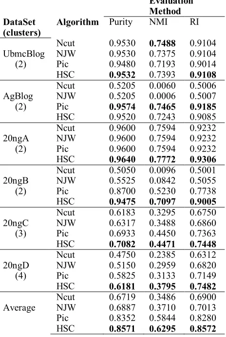
We compared the results of HSC against those of two state of the art spectral clustering methods Ncut (Shi and Malik 2000) and NJW (Ng, et al., 2001) and one recent method Pic (Lin and Cohen 2010) that uses truncated power iteration on a
normalized affinity matrix, see Table 1. HSC
scores highest on all text datasets, on all three evaluation metrics and just well on social network
data. The main reason for the effectiveness of HSC
is in its use of both local and global structure of the
graph. While the conditional probability
( ) ( )= ; ) looks at the immediate
transitions of state ( ), it uses for the target states which denotes a group of nodes that are being refined throughout the process. Using the stochastic matrix instead of embedding data points in the Eigen space or powering of the stochastic matrix may also be a contributing factor that demands future research.
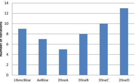
As for convergence analysis of the algorithm, we resort to EM’s convergence (Bormann 2004). The running complexity of spectral clustering methods is known to be of (| || |) (Chen and Ji 2010),
HSC is in ( | | ) where | |the number of
nodes, is the number of clusters and is the number of iterations to converge. Figure 1 shows the average number of iterations that HSC took to converge.
Table : Clustering performance of HSC and three
clustering algorithms on several datasets, for each dataset bold numbers are the highest in a column.
Evaluation Method DataSet
(clusters)
Algorithm Purity NMI RI
Ncut 0.9530 0.7488 0.9104 UbmcBlog NJW 0.9530 0.7375 0.9104 (2) Pic 0.9480 0.7193 0.9014
HSC 0.9532 0.7393 0.9108
Ncut 0.5205 0.0060 0.5006 AgBlog NJW 0.5205 0.0006 0.5007 (2) Pic 0.9574 0.7465 0.9185
HSC 0.9520 0.7243 0.9085 Ncut 0.9600 0.7594 0.9232 20ngA NJW 0.9600 0.7594 0.9232 (2) Pic 0.9600 0.7594 0.9232
HSC 0.9640 0.7772 0.9306
Ncut 0.5050 0.0096 0.5001 20ngB NJW 0.5525 0.0842 0.5055 (2) Pic 0.8700 0.5230 0.7738
HSC 0.9475 0.7097 0.9005
Ncut 0.6183 0.3295 0.6750 20ngC NJW 0.6317 0.3488 0.6860 (3) Pic 0.6933 0.4450 0.7363
HSC 0.7082 0.4471 0.7448
Ncut 0.4750 0.2385 0.6312 20ngD NJW 0.5150 0.2959 0.6820 (4) Pic 0.5825 0.3133 0.7149
HSC 0.6181 0.3795 0.7482
Ncut 0.6719 0.3486 0.6900 Average NJW 0.6887 0.3710 0.7013 Pic 0.8352 0.5844 0.8280
[image:4.612.310.542.297.642.2]Figure 1: Average number of iterations to converge
5 Conclusion and Future Work
We propose a novel and simple clustering method,
HSC, based on approximate estimation of the hard
assignments of nodes to clusters. The hard grouping of the data is used to simulate a probability distribution on the corresponding Markov chain. It is easy to understand, implement and is parallelizable. Experiments on a number of
different types of labeled datasets show that with a
reasonable cost of time HSC is able to obtain high
quality clusters, compared to three spectral clustering methods. One advantage of our method is its applicability to directed graphs that will be addressed in future works.
References
A. Kale, A. Karandikar, P. Kolari, A. Java, T. Finin and A. Joshi. 2007. Modeling trust and influence in the blogosphere using link polarity. In proceedings of the International Conference on Weblogs and Social Media, ICWSM.
A. Ng, M. Jordan, and Y. Weiss. 2001. On spectral clustering: Analysis and an algorithm. In Dietterich, T., Becker, S., and Ghahramani, Z., editors, Advances in Neural Information Processing Systems, pages 849–856.
B. Long, Z. M. Zhang, and P. S. Yu. 2007. A probabilistic framework for relational clustering. In KDD ’07: Proceedings of the 13th ACM SIGKDD international conference on Knowledge discovery and data mining, pages 470–479.
B. Poonen. 1999. Inequalities. Berkeley Math Circle.
C. D. Manning, P. Raghavan and H. Schu tze. 2008. Introduction to Information Retrieval. Cambridge University Press.
C. H. Q. Ding, X. He, H. Zha, M. Gu and H. D. Simon. 2001. A min-max cut algorithm for graph partitioning and data clustering. In Proceedings of ICDM 2001, pages 107–114.
F. Lin and W. Cohen. 2010. Power iteration clustering. ICML.
H. Jeong, S. P. Mason, A. L. Barabasi and Z. N. Oltvai. 2001. Lethality and centrality in protein networks. Nature, 411(6833):41–42
H. Kwak, C. Lee, H. Park and S. Moon. 2010. What is twitter, a social network or a news media? In Proceedings of the 19th international conference on World Wide Web, WWW ’10, pages 591–600.
I. Dhillon, Y. Guan, and B. Kulis. 2004. A unified view of kernel k-means, spectral clustering and graph cuts. Technical Report TR-04-25. UTCS.
J. Shi and J. Malik, 2000. Normalized cuts and image segmentation. IEEE Transactions on Pattern Analysis and Machine Intelligence, 22(8):888–905.
K. Macropol, T. Can and A. Singh. 2009. RRW: repeated random walks on genome-scale protein networks for local cluster discovery. BMC Bioinformatics, 10(1):283+.
L. A. Adamic and N. Glance. 2005. The political blogosphere and the 2004 U.S. election: divided they blog. In Proceedings of the 3rd international workshop on Link discovery, LinkKDD ’05, pages 36–43.
M. Meila and J. Shi. 2000. Learning segmentation by random walks. In NIPS, pages 873–879.
S. Bormann. 2004. The expectation maximization algorithm: A short tutorial.
S. Schaeffer, 2007. Graph clustering. Computer Science Review, 1(1):27–64.
S. M. van Dongen, 2000. Graph Clustering by Flow Simulation. PhD thesis, University of Utrecht, The Netherlands.
T. N. Bui and C. Jones, 1993. A Heuristic for Reducing Fill-In in Sparse Matrix Factorization", in Proc. PPSC, pp.445-452.
U. von Luxburg, 2007. A tutorial on spectral clustering. Statistics and Computing, 17(4):395–416.