Robust Scale Estimation for the Generalized
Gaussian Probability Density Function
Rozenn Dahyot
1and Simon Wilson
2Abstract
This article proposes a robust way to estimate the scale parameter of a gener-alised centered Gaussian mixture. The principle relies on the association of samples of this mixture to generate samples of a new variable that shows relevant distribu-tion properties to estimate the unknown parameter. In fact, the distribudistribu-tion of this new variable shows a maximum that is linked to this scale parameter. Using non-parametric modelling of the distribution and the MeanShift procedure, the relevant peak is identified and an estimate is computed. The whole procedure is fully auto-matic and does not require any prior settings. It is applied to regression problems, and digital data processing.
1
Introduction
Many problems in computer vision involve the separation of a set of data into two classes, one of interest in the context of the application and the remaining one. For instance, edge detection in images requires the thresholding of the gradient magnitude to discard noisy flat areas from the edges. The challenge is then to automatically select the appropriate threshold (Rosin, 1997).
Regression problems also involve the simultaneous estimation of the variance or stan-dard deviation of the residuals/errors. The presence of a large number of outliers makes difficult the estimation of the parameters of interest. Performance of robust estimators is highly dependent on the setting of a threshold or scale parameter, to separate the good data (inliers) that fit the model, from the gross errors (outliers) (Chen and Meer, 2003). The scale parameter, needed in M-estimation and linked to the scale parameter of the inliers residuals, is often set a priori or estimated by the Median Absolute Deviation. Ap-plications of robust regression (Chen and Meer, 2003) are, for instance, line fitting (Wang and Suter, 2004), or camera motion estimation (Bouth´emy et al., 1999). Those estimates also require the setting of a threshold (or scale parameter) to discard gross errors (outliers) from the relevant ones (inliers).
This paper proposes a solution for the estimation of the scale parameter that can be used iteratively along with location parameter estimation (Miller and Stewart, 1996; Chen and Meer, 2003; Wang and Suter, 2004) when there are many outliers, by assuming a
1School of Computer Science and Statistics, Trinity College Dublin, Ireland; [email protected]
mixture model. This method is based on the definition of two random variables Y and
Z computed from the samples of variable X using a non-linear transformation. The
distributions of those new variables have properties that allow us to define new estimates for the scale parameter. The computation of those new estimates requires us to detect a particular maximum over the distribution of the new variables. This is achieved using nonparametric kernel-based modelling of probability density functions. The resulting method is then both robust and unsupervised.
Section 2 presents related works. Section 3 presents our new estimates. Section 4 presents the computation. Paragraph 5 proposes to use this procedure for scale estimation iteratively with a location parameter estimation. Section 6 presents experimental results showing the robustness of the approach, and an application to robust object recognition.
2
Related works
Several works have been carried out on robust regression in the vision community (Stew-art, 1999), offering complementary views to statistics (Huber, 1981; Hampel et al., 1986). Wang has recently proposed a clear overview in both domains (Wang, 2004), underlining several differences. In particular, in the vision community, the breakdown point is usually expected far below 50% of outliers to deal with real world applications, and proofs of robustness are usually inferred through experimental results. In statistics, formal proofs of robust estimator properties usually prevail (even if those are only valid under strict assumptions that may never be encountered in practice) as it provides insights into the approaches (Hampel et al., 1986).
We consider the problem of robust regression:
v =f(u, θ) +
The mapping functionf is assumed to be described by the vectorθ (location parameter).
From a set of observations{(vi,ui)}, the goal of regression is to estimateθ.
Maximum likelihood is a popular estimation method. It relies on the modelling of
the probability density function of the residual that expresses the error between each
observation and its prediction by the mapping. Standard parametric modellings for the pdf of the residuals include Gaussian and Laplacian density functions (Hasler et al., 2003). Those models fail when gross errors or outliers occur in the observations. In this case, the pdf of the residuals can be expressed as a mixture:
P(|θ, σ) = P(|C, θ, σ)· P(C) +P(|C)· P(C) (2.1)
whereC is the inlier class for the model designed by the location parameterθ andσ the
scale parameter. The distribution of the inliersP(|C, θ, σ)is modelled by a parametric
distribution, e.g. centered Laplacian (Hasler et al., 2003) or Gaussian (Wang and Suter,
2004), depending on the location parameterθ to be estimated and the scale parameterσ
also usually unknown. Those parametric models usually offers a good description in real world applications.
the estimate. Weights are then a function of the residuals. The second approach consists in using sampling strategies and in estimating from several randomly selected subsets of observations. The final selection is then performed by comparing each estimate and keeping the optimal one. In a way, it can be seen as a similar approach to weighting the residuals in taking null weights on left out data at each round. However, this approach is different as weights are set randomly on data and do not depend on the values of the residuals. M-estimators or R-estimators are examples of objective functions that use a weighting strategy (Huber, 1981; Hampel et al., 1986). By their efficiency and their rather low computation cost, M-estimators in particular, have been widely applied to many computer vision applications such as camera motion estimation (Odobez and Bouth´emy, 1995), object class learning (la Torre and Black, 2001), object detection (Dahyot et al., 2004a) and recognition (Black and Jepson, 1998). Using sampling has been made popular by Fischler and Bolles with the RANSAC estimator (Fischler and Bolles, 1981). It has been successfully applied to camera calibration and image matching (Fischler and Bolles, 1981).
Both the M-estimator and RANSAC depend on the scale parameterσ that needs to
be robustly assessed along with θ. Statistical solutions for the scale estimate include in
particular the Median Absolute Deviation (Hampel et al., 1986) and Least Median Square (Miller and Stewart, 1996). Those methods have been used for online estimation from current observations. It can also be set by hand (Fischler and Bolles, 1981), or learned a priori off-line, and then set once and for all in the context of specific applications (Dahyot
et al., 2000; Hasler et al., 2003). For the modelling of the distribution of outliers,P(|C),
nonparametric representation using histograms have also been proposed (Hasler et al., 2003) to define a more dedicated M-estimator for image matching.
However, in most applications, the scale parameter cannot be inferred, and needs to be
estimated in parallel toθwith a much lower breakdown than50%. Recently several
strate-gies involving nonparametric representations of the distribution of the residualsP(|θ, σ)
have been proven efficient. For instance, Chen et al. (Chen and Meer, 2003) proposed to re-express the M-estimator objective function on the residuals, as a kernel density like estimator where the scale parameter is substituted by a bandwidth. After localising the main central peak, surrounding basins of attraction are detected heuristically and are used as thresholds to separate inliers from outliers. The segmented inliers are then processed
further to produce an estimate ofθ. Similarily in (Wang and Suter, 2004), the distribution
of the residuals is modelled using a nonparametric kernel modelling. The central peak is assumed to be corresponding to the inliers, and is isolated from the rest of the pdf using a Meanshift based algorithm searching for surrounding valleys. From this rough classi-fication, the scale parameter is then robustly estimated by computing the Median. This
two step scale estimation (TSSE) is coupled with a location parameter θ estimation in a
similar fashion to RANSAC (Fischler and Bolles, 1981).
in that peaks in the estimated distribution are directly related to the unknown parameters (Goldenshluger and Zeevi, 2004).
3
New estimates for
σ
Another approach for scale parameter estimation has been proposed in (Dahyot et al., 2004b) based on some properties of independent samples from a Gaussian distribution. Indeed assuming a Gaussian distribution for the inliers, the distribution of square root
of the sum of squares of several independent samples is a χ distribution that shows a
maximum directly related to the scale parameter. This approach is further studied in this article.
3.1
Assumptions
Let us define the random variable X that follows a two class mixture model. We call
inliers the data that belong to the class of interest: x ∈ C, and outliers the other data
x ∈ C. It is possible to make some relatively loose assumptions about the distribution
of the classC of interest, to allow its statistics to be estimated from an observed mixture
distribution PX(x)(Hasler et al., 2003). In this work, we assume the distribution of the
inliers to be a Generalized centered Gaussian (Aiazzi et al., 1999):
PX(x|C, σ) = 2Γ(α)1·α·βα exp
h
−|x|1/α
β
i
withβ =σ1/α·hΓ(3Γ(αα))i1/(2α)
(3.1)
Settingα= 1(Laplacian law) andα= 1/2(Gaussian law) in equation (3.1), are two
pop-ular hypotheses (Hasler et al., 2003; Dahyot et al., 2004b). Assuming the shape parameter
αknown, we focus on the estimation of the scaleσ.
3.2
Definition of new variables
The variables Z = Pn
n=1|Xn|1/α and Y = Zα are defined with independent random
variablesXnthat follow the same probability density function (3.1).
Forn= 1andZ =|X|1/α, the pdfP
Z(z|C)corresponds to the gamma distribution:
GZ|(α,β)(z) =
zα−1
Γ(α)·βαexp
−z
β
, z ≥0 (3.2)
Whenn>1, the variableZis then defined by the sum of i.i.d. variables that follow a
gamma distribution. Using the characteristic function of the gamma distribution Φ(t) =
(1−ıβt)−α, the characteristic function ofP
Z(z|C, σ)is:
ΦZ(t) =
n
Y
n=1
By Inverse Fourier transform, the p.d.f PZ(z|C, σ) is the gamma function GZ|(nα,β)(z).
From the distribution ofZ, it is easy to infer the pdf ofY:
PY(y|C, σ) =
y(n−1)
α·Γ(nα)·βnαexp
−y1/α β
, y ≥0 (3.4)
The maximum of the distributionsPZ(z|C, σ)andPY(y|C, σ)can be then computed
(ig-noring the solutionz = 0as a special case):
ZmaxC =β·(nα−1), nα >1
YmaxC = [(n−1)α β]α, n>1
(3.5)
Those maxima depend on the parameterσby definition ofβ (cf. eq. (3.1)).
3.3
New estimates for
σ
From equation (3.5), we propose to estimateσusing:
σZ = Znαmax−1C
αhΓ(3α) Γ(α)
i1/2
, nα >1
σY = (nY−max1)αC·αα
h
Γ(3α) Γ(α)
i1/2
, n>1
(3.6)
The maximum of the distributions ofY andZ has first to be located. This can be made
difficult by outliers occurring in the observations such that the observed distribution for
X is a mixture (as forY andZ):
PX(x|σ) = PX(x|σ,C)· PX(C) +PX(x|C)· PX(C) (3.7)
Depending on the proportion and the values of the outliers, the localisation of the maxi-mum needed in the estimation gets more difficult. We assume that the relevant maximaxi-mum
for the estimation is the closest peak to zero in the distributions PY(y|σ) and PZ(z|σ).
Note that robust estimation using M-estimator for Gamma distribution has been proposed in the literature (Marazzi A., 1996). But this nonparametric method is shown to be more robust in Section 6.
3.4
Remarks
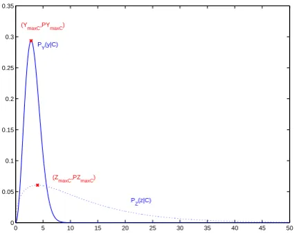
Figure 1 presents the pdfs of the inlier class for Y and Z. Instinctively, the higher the
maximum, the better its localisation should be in the mixture of observations. A priori,
considering the density of variable Y for the estimation of the scale parameter should
then perform better than the variable Z. However on the other hand, the transformation
from X to Z is spreading the range of variations of the observations, and consequently
decreasing locally the density of the outliers. Expressions of the maxima are given by:
PZ(ZmaxC|C, σ) = (nα−1)
nα−1
Γ(nα)·β exp [−(nα−1)]
PY(YmaxC|C, σ) = ((n
−1)α)(n−1)α
α·Γ(nα)βα exp [−(n−1)α]
0 5 10 15 20 25 30 35 40 45 50 0
0.05 0.1 0.15 0.2 0.25 0.3 0.35
PY(y|C)
(Y
maxC,PYmaxC)
P
Z(z|C)
(Z
[image:6.595.180.393.106.275.2]maxC,PZmaxC)
Figure 1:Probability density functionsPY(y|σ,C)andPZ(z|σ,C)(n= 3andα= 0.5).
4
Robust non-parametric estimation
Section 4.1 gives details on the computation of samples of the variableY andZ from the
samples of X. Paragraph 4.2 presents the nonparametric approach taken to perform the
computation of the relevant maxima in the estimation of the scale parameter.
4.1
Computing samples
From a set of observed independent samplesBx = {xi}i∈{1···i}, we need first to compute
the samplesBz ={zj}j∈{1···j} andBy ={yj}j∈{1···j} ofZ andY. It is performed by
ran-domly selectingnsamples fromBxto compute sampleszj andyj (Efron and Tibshirani,
1998). This should be done without replacement to insure independence of samples ofX.
However, ifiis large, it can also be performed with replacement.
It is assumed that the observed samples{zj} (or{yj}) are generated from a mixture
PZ(z|σ) of PZ(z|C, σ) (inliers) andPZ(z|C) (outliers). A priori, the proportion of the
inliers PY(C) in By and PZ(C) in Bz (i.e. when zj and yj are computed using xn ∈
C, ∀n ∈ [1;n]) is equal to (PX(C))n. However this proportion can be increased using
properties of the data. More precisely, audio and video data present strong spatio-temporal correlations that allow us to assume that data from a neighbourhood belong to the same
class (C or C) (Dahyot et al., 2004b). Using this assumption, samples for Y and Z are
carefully generated in order to limit the proportion of outliers by mis-coupling samples
of X. As a consequence, it is possible to compute samples of Y and Z such that the
proportion of inliers inBx, PX(C), is rather close to the proportions of inliers inBy and
4.2
Non-parametric estimation
4.2.1 Estimating distributions
From the collectionBy of samples ofY, a kernel estimate of the density functionPY(y)
can be computed:
ˆ
PY(y) =
1 i i X i=1 1
hyi ·k
y−yi
hyi
with k(·) chosen as a Gaussian N(0,1). The variable bandwidths {hyi}i=1···i are
se-lected automatically following Comanicciu et al. scheme (Comaniciu et al., 2001). The only change concerns the initial setting of the center point bandwidth: instead of the rule
of thumb plug-in, the more efficient Sheather-Jones plug-in bandwidth hSJ is computed
(Sheather, 2004).
4.2.2 Relation between bandwidths
For α = 12 (Gaussian distribution for the inliers), using the relation zi = yi2 between
samples in By and Bz, variable bandwidths are automatically computed for samples in
By, and then inferred for samples inBz by:
hzi =hyi·
q
4y2
i + 2hyi (4.1)
This relation betweenhziandhyiis derived by assuming a Gaussian variabley∼ N(yi, h
2
yi)
(from the kernel Gaussian assumption) and then by inferring the varianceh2
zi of the
vari-ablez = y2. For other values ofα, using the relationzi =y
1
α
i , the relation between the
bandwidths is approximated using first order Taylor series:
hzi =
1
α ·y 1
α−1
i ·hyi (4.2)
4.2.3 MeanShift
The closest mode to zero can be computed using mean shift from the minimum value of the samples (Dahyot et al., 2004b; Comaniciu et al., 2001):
Init y(0) = minyiBy
y(m+1) =
Pi
i=1hyi3
yig ˛ ˛ ˛ ˛
y(m)−yi
hyi ˛ ˛ ˛ ˛ 2! Pi
i=1h13
yi
g
„ y(m)−yi
hyi «
till convergenceYmaxC =y(m)
(4.3)
withg(t) = −k0(
√ t)
2√t . The same procedure is used to estimateZmaxC. Using equation (3.6),
5
Robust regression
For simplicity, we consider linear regression where observations Buv = {(vi, ui)}i=1···i
follow the linear mappingvi =uTi θ+i, ∀i. The joint estimation ofθandσis performed
by using the scale estimate introduced in the previous paragraphs, iteratively with a least
squares1estimation ofθperformed on a subsetSuvofpobservations (pis chosen superior
or equal to the dimension ofθ). This is similar to the RANSAC approach with an added
scale estimate. The algorithm can be described as:
• RepeatB times (see (Fischler and Bolles, 1981) for the choice ofB)
1. Select a subsetSuv(b) ofppoints randomly selected fromBuv,
2. Least Squares estimation of the location parameterθ(b)onSuv(b).
3. Compute the residuals{i =vi−uTi θ(b)}i=1···i, and samples ofY andZ.
4. Compute the bandwidths{hyi}and{hzi}as explained in Section 4.2.
5. Estimate the scale parameterσ(b)using procedure (4.3) and relations (3.6).
6. Compute the objective functionJ(b)(θ(b), σ(b)).
• Infer(ˆθ,σˆ)fromarg maxJ(b)(ouarg mindepending on the chosen objective
func-tion).
In this article, a similar objective function as Wang et. al has been chosen (Wang and Suter, 2004).
J(θ, σ) = Pi
i=11{|i|<2.5σ}
i·σ (5.1)
Note that, with our algorithm, a fixed θ leads to an estimate of σ, hence the space of
all possibilities(θ, σ)is not fully explored but only the space(θ, σθ). As a consequence
the objective function J has onlyθ as a variable. Some representations of the objective
function are presented in the experimental results in Section 6.2. Similarily to the Hough transform (Goldenshluger and Zeevi, 2004), the problem of recovering several models (or
multi-lines whenθis of dimensionp= 2) is to find all maxima (or minima) inJ.
6
Experimental results
Assessment of the robustness of the proposed method is done using simulations. Those simulations are performed under certain conditions explained below. That reflect real sit-uations of interest encountered in data analysis. In Section 6.1, two scenarios are tried : outliers with uniform distribution and pseudo-outliers with a Gaussian distribution. Re-sults for robust regression are reported in Section 6.2.
6.1
Scale estimate
In the following experiments, we chose α = 12, or a Gaussian distribution for the inliers,
i= 1000(cardinal ofBY andBZ), the groundtruth scale parameterσ = 2and the degree
of freedomn= 3:
• ∀n = 1,· · · ,n, setsBxnare used to compute setsByandBzsuch that the proportion
of inliers ∀n, PXn(C) = PY(C) = PZ(C). Outliers follow a uniform distribution
∀n, PXn(x|C) =U([−50; 50]).
• Pseudo-outliers follows a Gaussian distribution with the same variance as the inliers
and a mean µ. The proportion of the inliers is fixed such that ∀n, PXn(C) =
PY(C) =PZ(C) = 0.1.
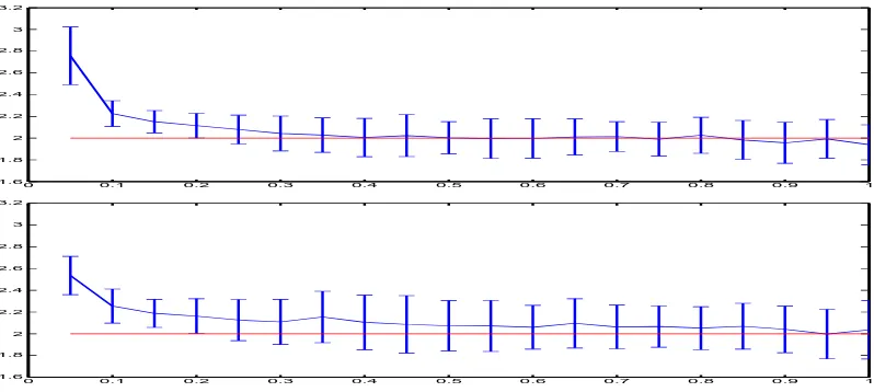
[image:9.595.87.486.415.594.2]6.1.1 Robustness to outliers
Figure 2 presents the mean of the estimates depending on the proportion of the inliers computed over 50 tries. As the proportion of inliers increases, the accuracy improves.
Althought σZ is less accurate than σY, it shows a better robustness to the proportion of
outliers. It is understood that the peak localisation for the estimation is easier performed
on the distribution ofZ thanY. In fact, when too many outliers occur, the inlier peak is
not anymore distinguishable in the pdf ofY.
0 0.1 0.2 0.3 0.4 0.5 0.6 0.7 0.8 0.9 1
1.6 1.8 2 2.2 2.4 2.6 2.8 3 3.2
0 0.1 0.2 0.3 0.4 0.5 0.6 0.7 0.8 0.9 1
1.6 1.8 2 2.2 2.4 2.6 2.8 3 3.2
Figure 2:Robustness to outliers: EstimatesσY (top) andσZ(bottom) with standard deviation, w.r.t. the proportion of inliersPY(C) =PZ(C). The red line corresponds to the
groundtruth scale parameter.
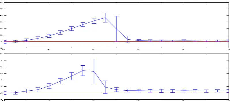
6.1.2 Robustness to pseudo-outliers
Figure 3 presents the mean of the scale estimates σY and σZ with standard deviation,
depending on the mean of the pseudo-outliers, computed over 50 tries. The estimate
σY is shown to be accurate when the mean µ of the pseudo-outliers is above3σ. The
0 1 2 3 4 5 1
2 3 4 5 6 7 8
0 1 2 3 4 5
[image:10.595.86.486.104.283.2]1 2 3 4 5 6 7 8
Figure 3:Robustness to pseudo-outliers: EstimatesσY (top) andσZ(bottom) with standard deviation, w.r.t. the mean of the Gaussian of pseudo-outliers expressed as a multiplicative of
σ(i.e. abscissa equal to 2 meansµ= 2σ).
PX(x|σ),PY(y|σ)andPZ(z|σ)for different values of the meanµof the pseudo-outliers.
The distributions are estimated using the kernel modelling as explained in Section 4.2. When the inlier and pseudo-outlier Gaussians are too close, their respective maxima are not anymore distinguishable.
6.1.3 Remarks
Similar results have been obtained for various inliers distribution i.e. different values of
α (in between 0.5 to 1) and n = 2,3. In practice, the choice of n should be as low as
possible to simplify the computation of samples ofY andZ.
6.2
Robust regression
In a similar experience as in (Wang and Suter, 2004), line parameters are estimated it-eratively with the scale parameter of the residuals (Miller and Stewart, 1996; Wang and Suter, 2004), following the procedure described in Section 5. Figure 5 shows the result of the estimation when 90% of outliers, uniformly distributed, appear in the observations.
This result has been obtained using the estimate σY and σZ. Several simulations have
been run on different randomly generated sets of observations. Ten estimates of the line are reported on the graph.
The previous experience is repeated with an added line of 50 points generated with
the equation u = v. Figure 6 shows the observations where alignements are barely
dis-tinguishable (left). Both lines can however be recovered in analysing maxima of the
objective function. Figure 7 presents the objective function J as a function of the
2-dimensional θ. Two peaks are clearly localised at the neighborhouds of θ = (1,0)and
θ = (−1,100), corresponding to the two lines coefficients. Numerically the first two
−6 −4 −2 0 2 4 6 8 10 12 0 0.02 0.04 0.06 0.08 0.1 0.12 0.14 0.16 0.18 0.2
−100 −5 0 5 10 15 0.02 0.04 0.06 0.08 0.1 0.12 0.14 0.16 0.18
−100 −5 0 5 10 15 20 0.02 0.04 0.06 0.08 0.1 0.12 0.14 0.16 0.18 0.2
0 1 2 3 4 5 6 7 8 9 0 0.05 0.1 0.15 0.2 0.25 0.3 0.35
0 2 4 6 8 10 12 14 0 0.05 0.1 0.15 0.2 0.25 pdf Y
0 2 4 6 8 10 12 14 16 18 0 0.05 0.1 0.15 0.2 0.25 0.3 0.35
0 20 40 60 80 100 120 140 160 180 0 0.002 0.004 0.006 0.008 0.01 0.012 0.014 0.016 0.018 0.02
0 50 100 150 200 250
0 0.002 0.004 0.006 0.008 0.01 0.012 0.014
0 100 200 300 400 500 600 700 0 1 2 3 4 5 6 7x 10
−3
[image:11.595.83.493.95.441.2]µ= 1.5σ µ= 2σ µ= 5σ
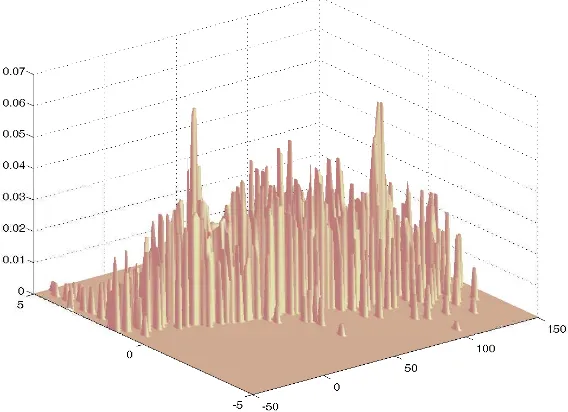
Figure 4:DistributionsPX(x|σ)(top) ,PY(y|σ)(middle),PZ(z|σ)(bottom). The relevant maximum for the estimation of the scale parameter becomes distinguishable afterµ >3σ.
0 10 20 30 40 50 60 70 80 90 100 0 10 20 30 40 50 60 70 80 90 100 Y
0 10 20 30 40 50 60 70 80 90 100 0 10 20 30 40 50 60 70 80 90 100 Z
Figure 5:Robust line fitting. Inliers: 50 points on a linex∈[0−100],u=−v+ 100and
σ = 1; Outliers: 450 points uniformaly distributed (Wang and Suter, 2004). The red line represents the groundtruth, and the green lines represent the estimates perform on 10 trials
[image:11.595.84.477.510.669.2]0 10 20 30 40 50 60 70 80 90 100 0
10 20 30 40 50 60 70 80 90 100
0 10 20 30 40 50 60 70 80 90 100 0
[image:12.595.82.474.107.259.2]10 20 30 40 50 60 70 80 90 100
[image:12.595.146.430.318.524.2]Figure 6:A two line fitting problem: Observations and estimated lines (green lines) with ground truth (red).
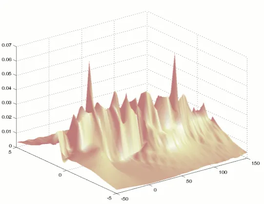
Figure 7:Objective function computed during the estimation. Two lines are present in the observations with parameterθ= (−1,100)andθ= (1,0). Both can be recovered by
localising the two main peaks.
Figure 7 presents the computed objective function as it is performed in the robust estimation proposed in paragraph 5. For comparison, we computed the objective function
for all values(θ, σ)on a finite domain and the graph is reported in figure 8.
6.3
Applications in computer vision
Figure 8:Simulated objective function.
A linear mapping is estimated by applying Principal Component Analysis (Dahyot et al., 2000) on 72 training colour images (image pixel values are arranged in a vector in lexicographic order) representative of an object class (cf. fig. 9). Eigenvectors associated with the highest eigenvalues summarize the informative visual content over the training
set. The representative eigenspace is chosen of dimension3for this experiment. Figure
[image:13.595.139.436.465.549.2]t0 t90 t180 t270
Figure 9:Example of training colour images for one object varying under different viewpoints (Nene et al., 1996).
10 presents the eigenbasis including the mean image and the first three eigenvectors. The
last image is the reconstruction of the templatet0performed on this basis. Considering an
20 40 60 80 100 120 20
40 60 80 100 120
20 40 60 80 100 120 20
40 60 80 100 120
20 40 60 80 100 120 20
40 60 80 100 120
20 40 60 80 100 120 20
40 60 80 100 120
20 40 60 80 100 120 20
40 60 80 100 120
µ
µµ u1 u2 u3 ˆt0
[image:13.595.82.450.658.731.2]unknown observation (image), its recognition consists in two tasks. The first is to estimate
its coordinate on the eigenspace (corresponding to the3-dimensional location parameter
θ). Then the recognition is completed by comparing this estimate with the coordinates
indexing the training images. The estimation problem can be written as follows:
Ri =µRi + (uRi )Tθ+Ri
Gi =µGi + (uGi )Tθ+Gi
Bi =µBi + (uBi )Tθ+Bi
(6.1)
where(Ri, Gi, Bi)are the colour values at the pixeliin the observed image, and(µRi , µGi , µBi )
and(uR
i ,uGi ,uBi )are the mean and the eigenvector values at pixel i(from the learning).
Residuals on each colour band are independent (n = 3). Noise is assumed Gaussian
(α= 0.5) and outliers typically occur because of a changing background or partial
occlu-sions.
The estimation ofθ is performed as described in Section 5. A comparison with
ro-bust recognition using M-estimators (Dahyot et al., 2000) is proposed and several results are presented in figure 11. Observations present the object with added Gaussian noise, different colour background and possible partial occlusions. The observations with a yel-low background (same yelyel-low as the main colour of the object itself) is tricky for the M-estimator based recognition method. In fact, M-estimation tries to match as many pix-els as possible in the observation and consequently matches templates with the highest number of yellow pixels. Our method however, with its objective function taking into ac-count both the scale and location parameter estimates from the current observation, gives a more accurate match for recognition.
7
Conclusion
The main idea of this article is to consider the generation of new variables whose distribu-tions show relevant properties for the estimation of an unknown parameter of the original variable. In particular, modes or maxima related to the unknown parameter can be lo-cated using non-parametric modelling. Accuracy of this estimation relies on the accuracy of the estimated density function, here performed by nonparametic modelling using ker-nels. The association with location parameter estimation performs very well in terms of robustness to outliers. The proposed method is fully automatic, one drawback being the
computation of samples of Y orZ that must be carefully done to limit the proportion of
outliers.
Acknowledgments
This work has been funded by the European Network Of Excellence on Multimedia
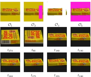
O1 O2 O3 O4
t270 t90 t180 t180
[image:15.595.141.435.100.351.2]t180 t175 t355 t180
Figure 11:Observations (top), recognition performed with M-estimators as in (Dahyot et al., 2000) (middle), recognition with simultaneous robust estimation of the scale and location
parameters (bottom).
References
[1] Aiazzi, B., Alparone, L., and Baronti, S. (1999): Estimation based on entropy
matching for generalized gaussian pdf modeling. IEEE Signal Processing Letters,
6.
[2] Black, M. J. and Jepson, A. D. (1998): Eigentracking: Robust matching and tracking
of articulated objects using a view-based representation. International Journal on
Computer Vision,26, 63–84.
[3] Bouth´emy, P., Gelgon, M., and Ganansia, F. (1999): A unified approach to shot
change detection and camera motion characterization. IEEE Transactions on
Cir-cuits and Systems for Video Technology,9, 1030–1044.
[4] Chen, H. and Meer, P. (2003): Robust regression with projection based
m-estimators. In International Conference on Computer Vision, 878–885, Nice,
France.
[5] Comaniciu, D., Ramesh, V., and Meer, P. (2001): The variable bandwidth mean shift
and data-driven scale selection. In International Conference on Computer Vision,
438–445, Vancouver, Canada.
[6] Dahyot, R., Charbonnier, P., and Heitz, F. (2000): Robust visual recognition of
colour images. In IEEE proceedings of the conference on Computer Vision and
[7] Dahyot, R., Charbonnier, P., and Heitz, F. (2004a): A bayesian approach to
ob-ject detection using probabilistic appearance-based models. Pattern Analysis and
Applications,7, 317–332.
[8] Dahyot, R., Rea, N., Kokaram, A., and Kingsbury, N. (2004b): Inlier modeling for
multimedia data analysis. In IEEE International Workshop on MultiMedia Signal
Processing, Siena Italy.
[9] Efron, B. and Tibshirani, R. J. (1998): An Introduction to the Bootstrap. Chapman
& Hall/CRC.
[10] Fischler, M. A. and Bolles, R. C. (1981): Random sample consensus: a paradigm for model fitting with applications to image analysis and automated cartography.
Commun. ACM,24, 381–395.
[11] Goldenshluger, A. and Zeevi, A. (2004): The hough transform estimator.The Annals
of Statistics,32.
[12] Hampel, F. R., Ronchetti, E. M., Rousseeuw, P. J., and Stahel, W. A. (1986): Robust
Statistics : The Approach Based on Influence Functions. John Wiley and Sons.
[13] Hasler, D., Sbaiz, L., S¨usstrunk, S., and Vetterli, M. (2003): Outlier modeling in
image matching. IEEE Transactions on Pattern Analysis Machine Intelligence, 25,
301–315.
[14] Huber, P. (1981): Robust Statistics. John Wiley and Sons.
[15] la Torre, F. D. and Black, M. J. (2001): Robust principal component analysis for
computer vision. InProceedings of the International Conference on Computer
Vi-sion, Vancouver, Canada.
[16] Leonardis, A. and Bischof, H. (2000): Robust recognition using eigenimages.
Com-puter Vision and Image Understanding,78, 99–118.
[17] Marazzi A., R. C. (1996): Implementing m-estimators of the gamma distribution.
Robust Statistics, Data Analysis, and Computer Intensive Methods, in Honor of Pe-ter Huber’s 60th Birthday, 277–297.
[18] Miller, J. V. and Stewart, C. V. (1996): Muse: Robust surface fitting using unbiased
scale estimates. InIEEE Conference on Computer Vision and Pattern Recognition,
300–306.
[19] Nene, S. A., Nayar, S. K., and Murase, H. (1996): Columbia object image
li-brary (coil-100). Technical Report CUCS-006-96, Department of Computer Sci-ence, Columbia University.
[20] Odobez, J.-M. and Bouth´emy, P. (1995): Robust multiresolution estimation of
para-metric motion models.Journal of Visual Communication and Image Representation,
[21] Rosin, P. L. (1997): Edges: saliency measures and automatic thresholding. Machine Vision and Applications,9, 139–159.
[22] Sheather, S. J. (2004): Density estimation. Statistical Science,19, 588–597.
[23] Stewart, C. (1999): Robust parameter estimation in computer vision.SIAM Reviews,
41, 513–537.
[24] Wang, H. (2004): Robust Statistics for Computer Vision: Model fitting, Image
Seg-mentation and Visual Motion Analyis. PhD thesis, Monash University, Clayton Vic-toria, Australia.
[25] Wang, H. and Suter, D. (2004): Robust adaptive-scale parametric model estimation
for computer vision. Transactions on Pattern Analysis and Machine Intelligence,
![Figure 5: Robust line fitting. Inliers: 50 points on a lineσ x∈[ 0 −100] u ,=− v +100 and=1 ; Outliers: 450 points uniformaly distributed (Wang and Suter, 2004)](https://thumb-us.123doks.com/thumbv2/123dok_us/1532320.696771/11.595.83.493.95.441/figure-robust-tting-inliers-points-outliers-uniformaly-distributed.webp)