Estimating the number of data clusters via the contrast
statistic
Yuriy Lyakh, Vitaliy Gurianov, Oleg Gorshkov, Yuriy Vihovanets
Department of Medical Biophysics, Medical Informatics and Biostatistics, National Medical University, Donetsk, Ukraine Email: [email protected], [email protected], [email protected], [email protected]
Received 13 September 2011; revised 7 November 2011; accepted 21 November 2011
ABSTRACT
A new method (the Contrast statistic) for estimating the number of clusters in a set of data is proposed. The technique uses the output of self-organising map clustering algorithm, comparing the change in de- pendency of “Contrast” value upon clusters number to that expected under a uniform distribution. A simulation study shows that the Contrast statistic can be used successfully either, when variables describing the object in a multi-dimensional space are inde- pendent (ideal objects) or dependent (real biological objects).
Keywords:SOM Neural Network; Clustering; Gap Statistic; Silhouette Statistic
1. INTRODUCTION
The first stage of data analysis is in its presentation. Cluster analysis can be used for analyzing of multi-di- mensional data set [1]. Cluster analysis groups objects based on the information found in the data describing the objects. The goal is that the objects in a group will be similar to one other and different from the objects in other groups. There are many different clustering tech- niques. One of them is the self-organizing map (SOM) [2] with its related extensions is the most popular artificial neural algorithm for use in unsupervised learning, clus-tering, classification and data visualization. One of the major challenges in cluster analysis is estimation of the optimal number of “clusters”.
There have been many methods proposed for estimat-ing the number of clusters: gap statistic [3], silhouette statistic [4], jump methods [5], prediction strength [6], methods based on mixture models and inference of Bayesian factors [7,8].
Nowadays this method and its like are widely used for solving various bio-medical problems. Thus, in paper [9] we are offered the method of features phenotype model- ing and iterative cluster merging using improved gap sta-
tistics. A Gaussian Mixture Model (GMM) is employed to estimate the distribution of each existing phenotype, and then used as reference distribution in gap-statistics. Applying of this algorithm proves very fruitful for image- based datasets.
In many of bio-medical issues we have to deal with a very large data set [10]. Considerable interest is studies in genes cauterization [11,12]. Thus, study [13] presents method of clustering analysis of large micro array data-sets with individual dimension-based clustering (CLIC), which meets the requirements of clustering analysis par-ticularly but not limited to large micro-array data sets. CLIC is based on a novel concept in which genes are clustered in individual dimensions first and in which the ordinal labels of clusters in each dimension are then used for further full dimension-wide clustering. CLIC enables iterative sub-clustering into more homogeneous groups and the identification of common expression patterns. The method in question enables to carry out a very sub- station analysis of data-sets; however its application is a laborious, full-time job.
While solving biological and especially medico-bio- logical problems we often face the problem of defining not only the optimal number of clusters which characterize this or that pathology, but also of estimating the number of independent factor attributes, i.e. decrease of space dimensionality. One of the reasons that cause it is a high cost of medical attention.
Exposing of strongly correlating attributes will make it possible to lessen the amount of attributes that are nec-essary for the analysis, and also to cut the number of medico-biological parameters, that characterize this or that pathology. The methods have enumerated don’t solve this problem.
only natural that these are the methods we used for the comparative analysis with our method. The second sec-tion presents the method descripsec-tion. The third contains the results of this method application.
2. METHOD
Let X be a set with N points in a m-dimensional data space. Data is distributed in k clusters (O1, O2, , Ok are centres of these clusters). We examine a C point, which belongs to the O0 cluster. Then we define the Contrast of C(Cr) by Eq.1
0
0 n
O C Cr
O C
(1)
where O C0 is Euclidean distance C to the centre it’s cluster, O Cn0 is Euclidean distance C to the nearest cluster besides its own nearest. Points with large , are well clustered, whereas those with small , tend to lie between clusters. Then we characterize quality of the division (k clusters) by Eq.2 (Contrastindex)
Cr Cr
1
1 Contrast
N
i i
Cr N
(2)Intuitively, when points concentrates in the cluster centres, Contrast (k) will have a high value, when points are distributed uniformly, this value will be low. It will enable us to make a conclusion about the efficiency of the division into the given number of clusters.
3. RESULTS
3.1. Uniform Dataset
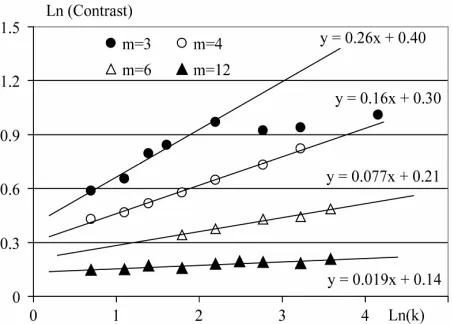
We generated datasets (10,000 points uniformly distrib-uted) in m-dimensional space. Then we divided data in k clusters, using SOM technique. Then we calculated Con-trast (k) of the division. Figure 1 presents results of the calculation for m = 3, 4, 6, 12 and k = 2, 3, , 64.
The following conclusions can be formulated from this analysis (Figure 1):
1) In the situation of uniformly distributed points (under condition of not great clusters number) dependence Con-trast index upon clusters number is described by Eq.3:
Contrast a k (3) where a and are constants.
2) (Eq.1) is a positive value and it decreases when dimension of space m increases.
3) When clusters number are great (for the given di-mension of space m) the Contrast index doesn’t depend on k (Contrast = Const).
[image:2.595.310.536.342.504.2]3.2. Computational Implementation
Figure 2 represents an example of Contrast statistic cal- culation. Five clusters in 4-dimensional space were simu-
lated (total 10,000 points). Contrast indexes for k = 2, 3, , 36 clusters were calculated.
The algorithm optimal number of clusters computation can be proposed:
1) Cluster the observed data, varying the total number of clusters from k = 1, 2, , K, calculating Contrast (k). 2) Obtain the regression line (ln(Contrast) vs ln(k)), which corresponds to uniform distribution, using great k values.
3) Estimate dimension of space number via line slope. 4) Finally choose the optimal number of clusters via Contrast (kopt) greatest deviates from the regression line.
3.3. Contrast Statistic and the Others Techniques
[image:2.595.311.537.555.698.2]There have been many methods proposed for estimating the optimal number of clusters: Gap statistic [3], Silhou- ette statistic [4] and so on. In the case of [3] with a large number of model examples the effectiveness of the pro- posed by author Gap statistics is most convincingly
Figure 1. Results for uniformly distributed points in m-dimen- sional space. The functions y(x) are shown (y = ln(Contrast), x = ln(k)).
demonstrated. For application of this approach in the case of k-means the value is calculated by Eq.4,
*
* ln ln 1 1 X X X XMSE k MSE k
g k MSE MSE (4) where
X*
MSE i —average Euclidean distance from the object to the centre of its cluster in the case of objects distribution under analysis in i-cluster (the quantity of objects in the referent distribution being equal to those the distribution under analysis ). In [3] we presume to compute the
X*
MSE i
g kvalue for several reference samples on the basis of which we calculate the average value and compute the standard deviation of this value sd (i).As the optimal clusters number such a minimal k is chosen, for which g k
1
sd k
1
[3].While computing Silhouette statistics [4] in the case of cauterization by method of average k, for every j-object of the distribution under analysis the value is calculated by Eq.5.
b j
a j s jb j
(5)
where a(j) is the average Euclidean distance from the objects to the other objects of the same cluster, b(j) the average Euclidean distance from the object to the objects of the nearest cluster, to which it doesn’t belong. The optimal number of clusters k should be considered as such, for which the average (for all the objects) values s(j) is maximal.
Further on we demonstrate the comparative analysis of application for the optimal cluster number selection the Contrast statistic, the Gap statistic and the Silhouette statistic.
For estimation the Contrast statistic efficiency we analyze some datasets:
1) Datasets simulated in a multi-dimensional space (independent variables), small and large point’s number.
2) Datasets simulated in a multi-dimensional space (dependent variables), small and large point’s number.
3) Practical datasets (real medical and biological data, dependent variables), small and large point’s number.
We applied three different methods for estimating the optimal number of clusters: Gap statistic, Silhouette sta-tistic, Contrast statistic.
The following results can be formulated:
1) For independent variables the Gap statistic is an ef-ficient method of optimal clusters number calculation. The similar results give both Silhouette statistic and Con- trast statistic.
2) For dependent variables the Gap statistic isn’t the efficient method. There is a problem on generation of reference distribution (unknown true number of space di-
mension). Both Silhouette statistic and Contrast statistic can be efficiently used.
3) Total time of Silhouette statistic calculation is as square of cluster size, total time of Contrast statistic cal-culation is as cluster size.
4) Additionally Contrast statistic allows estimating dimensional number of space for dependent variables (slope the regression line, using great k values) however one of the shortcomings of the estimation is that it is possible only with a small number of independent variables (m < 12).
3.4. Examples
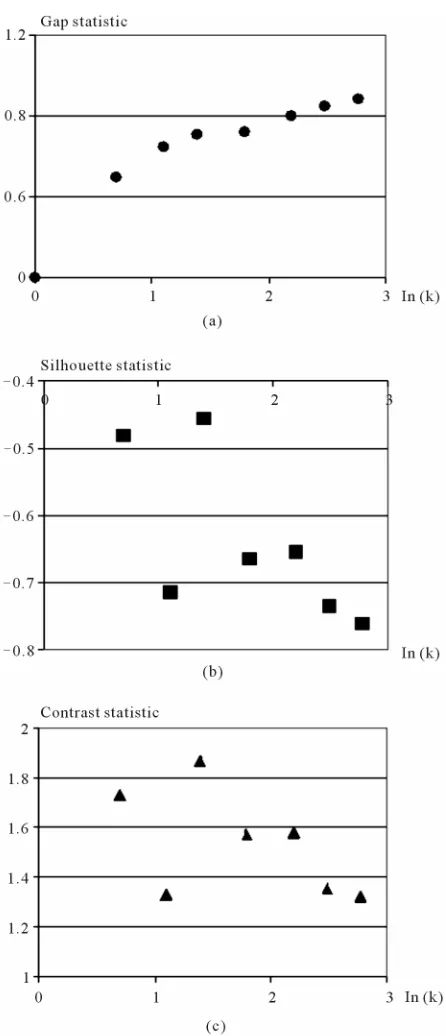
There are measurement data for 150 irises specimen, in equal parts (50 specimen each) belonging to three spe-cies (iris setosa, iris versicollor, iris virginica) [14]. For each iris specimen 4 parameters are known. Sepal length, sepal width, petal length, petal width. The task was first set by Fisher and its frequently used in mathematical statistics as a test-trial. While performing the correlation analysis the correlation connection for all the coordinates has been revealed. For finding out the minimal clusters number of this objects set the above proposed method has been applied. The set has been consequently broken up into 1, 2, , 16 clusters, and for each of these cases Gap statistic, Silhouette statistic, Contrast statistic have been calculated. Figure 3 presents results of the calcula-tion.
Analysis performed for the model task indicates that Gap statistics, Silhouette statistic and Contrast statistics all define the optimal cluster number as equaling to four.
A substantial analysis for each one of the separated clusters clearly demonstrates the biological importance of the solution obtained. In addition to the obtained op- timal clusters number, considering the Contrast index dependency on k, we may safely assume, that the number of independent variables, in which the mentioned objects are distributed, is close to 3.
Contrast statistics method was used for analysis of Data of the National Insulin-treated Diabetics Register [15]. Clustering was conducted on a 6324 patients data holding sample. During the SOM mapping, the number of clusters varied from 25 to 3. The clearest data repre- sentation structure turned out to be with 3 clusters.
Figure 3. The results of analysis of Ln statistics index depend-ency of the Ln number of division clusters of the Fisher’s Irises example (4—dimensional space, 3 kinds of flowers) (a) Gap statistic; (b) Silhouette statistic; (c) Contrast statistic.
serious” related to the 3rd cluster. The 2nd cluster con-tained modest cases [15].
4. CONCLUSION
New Contrast statistic technique the number of data clusters estimation is proposed. The method can be
efficiently used for the real large medical and biological dataset. Contrast statistic additionally allows estimating dimen- sional number of space (only in the case of small space dimentionality) for dependent variables.
REFERENCES
[1] Behbahani, S. and Nasrabadi, A. (2009) Application of SOM neural network in clustering. Journal Biomedical Science and Engineering, 2, 637-643.
doi:10.4236/jbise.2009.28093
[2] Kohonen, T. (1982) Self-organized formation of topolo- gically correct feature maps. Biological Cybernetics, 43, 59-69. doi:10.1007/BF00337288
[3] Tibshirani, R., Walther, G. and Hastie, T. (2000) Estimat-ing the number of cluster in a dataset via the gap statistic. Technical Report, Department of Biostatistics, Stanford University, Stanford.
[4] Dudoit, S. and Fridlyand, J. (2002) A prediction—Based resampling method for estimating the number of clusters in a dataset. Genome Biology, 3,1-21.
doi:10.1186/gb-2002-3-7-research0036
[5] Sugar, C. and James, G. (2003) Finding the number of clusters in a dataset: An information-theoretic approach.
Journal of the American Statistical Association, 98,750- 763. doi:10.1198/016214503000000666
[6] Tibshirani, R. and Walther, G. (2005) Cluster validation by prediction strength. Journal of Computational & Gra- phical Statistics, 14,511-528.
doi:10.1198/106186005X59243
[7] Guo, P., Chen, P. and Lyu, M. (2002) Cluster number selection for a small set of samples using the Bayesian Ying-Yang model. IEEE Transactions on Neural Net-works, 13, 757-763. doi:10.1109/TNN.2002.1000144 [8] Gangnon, R. and Clayton, M. (2007) Cluster detection
using Bayes factors from over-parameterized cluster mo- dels. Environmental and Ecological Statistics; 14, 69-82. doi:10.1007/s10651-006-0007-7
[9] Yin, Z., Zhou, X.B., Bakal, C., Li, F.H., Sun, Y.X., Per-rimon, N. and Wong, S.T.C. (2008) Using iterative cluster merging with improved gap statistics to perform online phenotype discovery in the context of high-throughput RNAi screensBMC. Bioinformatics, 9, 264.
[10] Sharma, A., Podolsky, R., Zhao, J. and McIndoe, R.A. (2009) A modified hyperplane clustering algorithm allows for efficient and accurate clustering of extremely large datasets. Bioinformatics, 25, 1152-1157.
doi:10.1093/bioinformatics/btp123
[11] Medvedovic, M. and Sivaganesan, S. (2002) Bayesian infinite mixture model based clustering of gene expres-sion profiles. Bioinformatics, 18, 1194-1206.
doi:10.1093/bioinformatics/18.9.1194
[12] Qin, Z.S. (2006) Clustering microarray gene expression data using weighted Chinese restaurant process. Bioin-formatics, 22, 1988-1997.
doi:10.1093/bioinformatics/btl284
CLIC: Clustering analysis of large microarray datasets with individual dimension-based clustering. Nucleic Acids Research, 38, W246-W253.doi:10.1093/nar/gkq516 [14] Kim, J.H., Kohane, I.S. and Ohno-Machado, L. (2002)
Visualization and evaluation of clusters for exploratory analysis of gene expression data. Journal of Biomedical Informatics, 35, 25-36.
doi:10.1016/S1532-0464(02)00001-1