Gravitons into Gravitational Field

(1)

ISSN Online: 2380-4335 ISSN Print: 2380-4327

DOI: 10.4236/jhepgc.2018.44039 Oct. 11, 2018 695 Journal of High Energy Physics, Gravitation and Cosmology

Gravitons into Gravitational Field

Andrey N. Volobuev

Department of Medical Physics, Samara State Medical University, Samara, Russia

Abstract

The problems connected to propagation of a gravitational field are consi-dered. The constant homogeneous gravitational field is investigated. The law of electromagnetic radiation frequency change in this gravitational field is shown. On the basis of the solution of the Einstein’s equation for a weak gra-vitational field, the flux of gragra-vitational radiation energy from system of coo-perating masses is found. The equation for gravitational waves is found. On the basis of refusal from a stresses tensor into energy-impulse tensor and use of a quantum gravitational eikonal, the quantum form of the energy-impulse tensor in Einstein’s equation is found. The equation for a graviton propagat-ing in a gravitational field of a double star is found. Resonant interaction of a graviton and a gravitational field of a double star are investigated. It is shown that such interaction allows registering the gravitons.

Keywords

A Gravitational Eikonal, Metric Tensor, Einstein’s Equation, Energy Flux, Gravitational Waves, Energy-Impulse Tensor, Registration of Gravitons

1. Introduction

The modern theory of gravitation—the theory general relativity of Einstein—is a basis for calculation of the astrophysics phenomena. It is generalization Newto-nian dynamics, including the law of universal gravitation. As well as NewtoNewto-nian dynamics the theory general relativity is not the quantum theory. The Einstein’s equation for a gravitational field does not have stochastic nature. It contradicts modern physics. For example, for an electron cooperating with a gravitational field with help of the Einstein’s equation, it is possible to calculate position ab-solutely precisely that contradicts a principle of Heisenberg’s uncertainty.

Obviously such situation is unacceptable however the problem of a gravita-tional field quantization till now is not solved though for the solving of this

How to cite this paper: Volobuev, A.N. (2018) Gravitons into Gravitational Field. Journal of High Energy Physics, Gravita-tion and Cosmology, 4, 695-715.

https://doi.org/10.4236/jhepgc.2018.44039

Received: August 31, 2018 Accepted: October 8, 2018 Published: October 11, 2018

(2)

DOI: 10.4236/jhepgc.2018.44039 696 Journal of High Energy Physics, Gravitation and Cosmology

problem many efforts have been applied [1] [2] [3] [4].

Recently the problem of gravitational waves detecting which description is possible with the help of the Einstein’s equation of general relativity is solved. The further increase of sensitivity of a measuring method will allow estimating more adequately correctness and other alternative theories of gravitation [5].

From the physical point of view the general relativity theory assumes that the mass curvature is a space-time [6]. This curvature of space-time influences all particles moving in space, including and what creates a curvature. Influence is carried out and on massless particles, for example-photons. It is connected to a curvature of geodetic lines of space-time on which photons move. Space-time curvature in the general relativity theory identifies with occurrence of some gra-vitational fields due to which there is an interaction of mass particles. Photons also change the frequency in a gravitational field.

Gravitational waves are propagating oscillations of the curved space-time as similar as the waves on a water surface are propagating oscillations of the water particles.

However in the submitted physical picture of gravitation there is no the major element—quantization of a gravitational field.

Attempts to solve a problem of the gravitational waves quantization with the help of 5-dimensional space-time use [7] can hardly lead to success. Apparently, the theory of 5-dimensional space-time now has only a historical value. By comparison of distance from the source of gravitational waves calculated by the attenuation of experimentally registered gravitational waves and by the red dis-placement of electromagnetic radiation it has been established [8] that dimen-sion of our space-time is equal ~ 4 0.1± _{. Thus our space-time is described by}

four coordinates: time and three spatial coordinates.

Assuming as a whole correctness of the Einstein’s equation for a gravitational field we research some features of a gravitational radiation and quantization of the gravitational waves.

2. Photon in Constant Homogeneous Gravitational Field

For the beginning we shall consider how frequency of an electromagnetic radia-tion quantum (photon) in a constant homogeneous gravitaradia-tional field changes. Research we shall carry out in flat space-time the name Minkowski’s space. The interval in inertial reference system looks like [6]:

( )

2 2 2 2 2 2

2 2 2 2

0 1 2 3

00 11 22 33

d d d d d

d d d d

s c X Y Z

g X g X g X g X

τ

= − − −

= − − − (1)

where designations there are _{X X Y X Z X}₌ 1_, ₌ 2_, ₌ 3_{—the Cartesian}

coordi-nates, c—a light velocity in vacuum, d

τ

_{—an interval proper time between}

events [6], so _c_d_{τ =}_d_X0_,

00 1, 11 22 33 1

g = g =g =g = − _{—the metric tensor}

(3)

DOI: 10.4236/jhepgc.2018.44039 697 Journal of High Energy Physics, Gravitation and Cosmology 0

00

1

d g Xd

с

τ= (2)

As it will be shown further in a gravitational field g00<1. Therefore, proper

(or own) time flows that more slowly than is less g00 in the given point of

space (∆ =τ τ2−τ1 decreases; τ2 in field it is less τ2 outside of field). The

clock per a gravitational field is slow.

A function of Lagrange of a particle in the gravitational field looks like [6]:

2 2

1

1 1

2

g g

V V

L T U mc m mc m

c ϕ c ϕ

 

= − = − − − = − _ − _−

  (3)

where m there is mass of a particle in a field, V—its velocity, ϕg—gravitational

potential of a field, so acceleration V= −gradϕ_g.

Action for a particle in a gravitational field is equal [6]:

2

d d d

2

g V

S L mc c mc s

c c

ϕ

τ

 

τ

= = − _ − + _ = −

 

∫

(4)

where S there is the action for a free material particle, ds—interval. Hence, the square of the interval ds is equal:

2 2

2

2 2 2 2 2

2

2 2

2 2 2 2 2 2

2 4 2

d d 2 d

2

1 2 d d 1 d d

g g

g

g g g

V

s c c V

c c c

c c

c c c

ϕ ϕ

τ ϕ τ

ϕ ϕ ϕ

τ τ

 

= − +  =_ − + + _

   

   

= _ + + _ − =  +  −

 

  r r

(5)

where it is used dr V= d

τ

.

Thus according to (1) the component of metric tensor g00 in a gravitational

field decreases:

2

00 1 2

g

c

ϕ

 

= + 

  and 00 1 2

g g

c ϕ

= + (6)

where ϕg there is negative size.

For the further analysis we use concept of an eikonal [6]. Eikonal there is a phase of the periodic function describing a field of electromagnetic wave:

φ

=kq−

δτ

(7) where k there is a wave vector of an eikonal, q-a coordinate vector of an eikonal (it is optional Cartesian), δ-cyclic frequency of the eikonal.

Taking into account (2) and (7) it is possible to find the eikonal frequency (a photon frequency in the given point in a proper time):

0

0 0

00

X c

X g X

φ

δ

τ

∂ ∂ ∂ ∂

= − = − = −

∂ ∂ ∂ ∂ (8)

If to use the world time t (outside of a gravitational field), so that t X0 c

= the

photon cyclic frequency measured in world time is equal 0 _t c _X0

φ φ

(4)

Hence, according to (8) with the account (6) we have:

0 0

00

2

1 g

g

c

δ δ

δ = = _ϕ

+ (9)

where

δ

0 there is photon frequency at absence of a gravitational field.

Thus, photon frequency depends on size of a gravitational field potential. As the gravitational field potential it is negative size at approach to the creating a field bodies, the photon frequency

δ

grows, and at removal falls (red dis-placement). For example, for a body in mass M the potential of a field depends on radius r under the formula ϕg= −kM_r .

The eikonal wave vector (or a photon wave vector) =∂φ ∂ k

q , and 4-impulse in

the Cartesian coordinates is equal i i k

X φ ∂ = −

∂ . But for the 4-impulse the formula

0 0 ₀

i i

k k =k k −kk= is correct. Hence, _i 0

i X X

φ φ

∂ ∂ ₌

∂ ∂ there is the eikonal

equa-tion.

Let’s note that the eikonal is a quantized size. The eikonal quantum is equal:

0

S =_φ₍₁₀₎

where



there is reduced Planck’s constant.

3. Generating of a Gravitational Radiation, and Gravitational

Waves

Gravitational radiation arises at the relative movement of massive bodies. We shall consider the weak gravitational radiation created by the rather small bodies which move with small velocities.

Let’s assume that gravitational waves are connected to small change of a me-tric tensor. In this case it is possible to write down [6]:

( )0

ik ik ik

g =g +h ₍₁₁₎

where ( )0

ik

g there is basic part of a metric tensor created by a body, hik—the

small gravitational additive of a metric tensor concerning to the radiated waves, so ( )0

ik ik

g h .

The gravitational field is described by the Einstein’s equation. For writing of the Einstein’s equation it is necessary, first of all, by the mathematical to describe a curvature of space-time. For the description of the mathematical curvature of space-time it is used a tensor of curvature (Riemann’s tensor) [6]:

(

)

Гi Гi _{Г Г} _{Г Г}

i n i n

km kl

iklm l m nl km nm kl

R

X X

∂ ∂ 

=_ − _+ −

∂ ∂

  (12)

where Гi

kl there is a projection of a derivative unit vector ek on coordinate l

X on a coordinate axis _Xi_{—Cristoffel’s symbol}_Гi k kl i l

e e

X

∂ =

(5)

symbols it is the functions of coordinates characterizing change a component of a vector at its parallel displacement. All indexes, bottom (covariant, usually functional sizes) and top (contravariant, usually coordinate sizes) accept values 0 (a time index), 1, 2, 3 (coordinate indexes). As it is usual summation is carried out on indexes repeating in products.

Cristoffel’s symbols can be expressed through metric tensor [6]:

1

Г

2

i im mk ml kl

kl l k m

g g g

g

X X X

∂ ∂ ∂

 

= _ + − _

∂ ∂ ∂

  (13)

Thus curvature tensor of a space-time it is determined by a velocity and ra-pidly of a metric tensor gik change in the space-time. Generally there are 10

components of a metric tensor: 4 - with identical indexes (00, 11, 22, 33), and 6 with different indexes (01, 02, 03, 12, 13, 23, 2

4 4 3 6_{1 2}

С = × = × ).

The curvature tensor is a fourth rank. Physically the curvature of space-time can be described only the second rank tensor since energy—impulse tensor creating this curvature is the second rank tensor. Therefore we shall pass with the help of a curtailing operation in (12) to the second rank tensor (Ricci’s ten-sor):

(

)

Гl Гl _{Г Г} _{Г Г}

lm ik il l m m l

ik limk l k ik lm il km

R g R

X X

∂ ∂ 

= =_ − _+ −

∂ ∂

  (14)

The Ricci’s tensor it is symmetrical:

ik ki

R =R ₍₁₅₎

Further we shall introduce a scalar curvature of a space-time under the for-mula:

ik ik

R g R= ₍₁₆₎

where _gik_{there is contravariant metric tensor.}

Using the Ricci’s tensor (14), a scalar curvature of a space-time (16), and also a metric tensor gik, the Einstein has written down the basic equation for a

gra-vitational field:

4

1 8π

2

ik ik k ik

R g R T

c

− = (17)

The left part of this equation refers to Einstein’s tensor 1 2

ik ik ik

E =R − g R_{. It}

characterizes geometrical properties of a space-time in particular its curvature. The right part of the equation includes an energy-impulse tensor of the second rank describing the source which creates the curvature of a space-time:

00 01 02 03 10 11 12 13 20 21 22 23 30 31 32 33

ik

T T T T

T

T T T T

 

 

=

 

 

(18)

(6)

1 8π

2

ik ik ik

ik ik k ik

g R g g R g T

c

− = (19)

Taking into account ik

ik

R g R= and ik 4

ik

g g = (in a four-dimensional

space-time) we shall find:

4 4

8π _Sp 8π

ik

k k

R T T

c c

− = = (20)

where it is designated SpTik =T .

Having substituted (20) in the Einstein’s Equation (17) we shall find:

4

8π 1

2

ik k ik ik

R T g T

c

 

= _ − _

  (21)

Outside of a spherical symmetric body in mass M creating a gravitational field the energy-impulse tensor is equal to zero Tik= =T 0. In this case according to

(21):

0

ik

R = ₍₂₂₎

Zero size of the Ricci’s tensor according to the Equation (22) does not mean that there is no curvature of a space-time. The space-time curvature which is characterized by the Riemann’s tensor (12) is kept in distance from the bodies creating this curvature.

Let’s substitute the Cristoffel’s symbols (13) in the first bracket of a Riemann’s curvature tensor (12) of space-time. In result we have:

(

)

2 2 2 2

1 _{Г Г} _{Г Г}

2

n p n p

im kl km il

iklm k l i m i l k m np kl im km il

g g g g

R g

X X X X X X X X

 ∂ ∂ ∂ ∂ 

= _ + − − _+ −

∂ ∂ ∂ ∂ ∂ ∂ ∂ ∂

  (23)

In the Formula (23) we shall substitute (11), and neglecting for the small gra-vitational additive hik the products of the Cristoffel’s symbols we shall find:

2 2 2 2

1

2 im kl km il

iklm k l i m i l k m

h h h h

R

X X X X X X X X

 ∂ ∂ ∂ ∂ 

= _ + − − _

∂ ∂ ∂ ∂ ∂ ∂ ∂ ∂

  (24)

Let’s pass to the Ricci’s tensor multiplying (24) at the left on not perturbed metric tensor _g( )0lm_{. Taking into account:}

( )

(

0

)

(

( )0ik

)

( ) ( )0 0ik ( )0ik ( )0 ( ) ( )0 0ik

ik ik ik ik

ik ik ik ik ik ik ik ik

g g = g +h g −h =g g +h g −g h −h h ≈g g

for contravariant components as against (11) it is possible to write down ap-proximately (product of additives to metric tensor it is neglected):

( )0lm

lm lm

g =g −h (25)

Thus we shall find:

( )0 2 2 2 2

1 2

l l

lm ik i k

ik l m k l i l i k

h h h h

R g

X X X X X X X X

 ∂ ∂ ∂ ∂ 

= − _{∂ ∂} +_{∂ ∂} +_{∂ ∂} −_{∂ ∂} 

  (26)

where it is designated i i

h h= . Rise of indexes was carried out by a rule

( )0kl k

i il

h =g h .

(7)

2 l 2 l 2

i k

k l i l i k

h h h

X X X X X X

∂ ₊ ∂ ₌ ∂

∂ ∂ ∂ ∂ ∂ ∂ (27)

Let’s show that a condition (27) is gauge condition. We shall transform the left part:

2 2

l l l l l l

i k i k i i

k l i l l k i l k k l

h h h h h h

X X X X X X X X X X X

     

∂ ₊ ∂ ₌ ∂ ∂ ₊ ∂ ₌ ∂ ∂ ₌ ∂ ∂

     

∂ ∂ ∂ ∂ ∂ _∂ ∂ _ ∂ _∂ _ ∂ _∂ _ (28)

Equating (27) and (28), we shall find:

2 il

i l

h

h _const

X X

∂

∂ ₌ ₊

∂ ∂ (29)

If scalar curvature of space due to the gravitational additive of metric tensor is small h→0, and accepting a constant of integration equal to zero that is reached by a choice of the reference system beginning, we receive:

0 1 2 3 0

1 2 3 div 0

l

i i i i i i

i l

h h h h h h

ct ct

X X X X

∂ ₌∂ ₊ ∂ ₊ ∂ ₊ ∂ ₌∂ ₊ ₌

∂ ∂

∂ ∂ ∂ ∂ h (30)

The received condition is similar to Lorentz’s gauge in electrodynamics. Therefore equality (27) is a gauge condition.

Thus Ricci’s tensor (26) with the account (27) looks like:

( )0 2 2 2

2 2

1 1 1

2 2

lm ik ik ik

ik l m

h h h

R g

X X

X X α α c t

 ∂   ∂ ∂ 

= − _{∂ ∂} = _{∂ ∂} − _∂ 

    (31)

Let’s substitute the received expression of the Ricci’s tensor (31) in Einstein’s equation for a gravitational field as (21). In empty space outside the mass creat-ing a gravitational field we shall assume the diagonal components of ener-gy-impulse tensor equal to zero

T

=

0

. In this case we have:

2 2

2 2 4

1 16π

ik ik

ik

h h _{k T}

X Xα α c t c

∂ ∂

− =

∂ ∂ ∂ (32)

The solution of the Equation (32) is well-known from the theory of retarded potentials [10]. At small speeds of movement of a gravitational radiation source:

0 4

0

4 _d

ik ik

V

r k

h T t V

c c r

 

= − _ − _

 

∫

(33)

where r0 there is distance from the mass center of a field source up to a point

of supervision, V - volume on which integration is carried out.

Let’s find a derivative of the left and right parts of the Equation (31) on Xk:

( )0 2

4

1 8π

2

lm

ik ik ik

l m

k k k

R _g h k T

X X X X c X

  

∂ ₌ ₋ ∂ ∂ ₌ ∂

  

 

∂ _ ∂ ∂ _∂ __ ∂ (34)

Taking into account (30) at replacement of an index l on an index k, we have:

0

ik

k T X ∂

=

∂ (35)

(8)

Let’s write down the Equation (35) having allocated a time component:

0 0 0 T T X X αγ α γ ∂ ₋∂ ₌

∂ ∂ and

0 00 0 0 T T X X γ γ ∂ ₋∂ ₌

∂ ∂ (36)

Let’s multiply the first Equation (36) on Xβ_{and we shall integrate it on all}

space:

(

)

0

0 d d d d d

T X T

T X V X V V T V T V

X X X

β αγ αγ

β β

α γ γ αβ αβ

∂ ∂

∂ ₌ ₌ ₋ _{= −}

∂

∫

∂

∫

∂

∫

(37)

where according to Gauss’s theorem

(

T X

)

dV

(

T X

)

dS 0

X β αγ β αγ γ ∂ = = ∂

∫

_

∫

for

0

Tαγ = _{on infinity.}

The equality (37) can be copied in a symmetrical kind:

(

0 0

)

0

1

d d

2

T V T X T X V

X

β α

αβ α β

∂

= − +

∂

∫

(38)

Similarly we shall multiply the second Equation (36) on X Xα β_{and we shall}

integrate it on all space:

(

)

0 00 0 0 0 0 d d

d d d

T

T X X V X X V

X X

T X X

V T X V T X V

X

γ

α β α β

γ

α β

γ _β _α

α β γ ∂ ∂ ₌ ∂ ∂ ∂ = − − ∂

∫

(39)

From (39) follows:

(

)

00 0 0

0 T X X Vd T X T X dV

X

α β β α

α β

∂ _{= −} ₊

∂

∫

(40)

Substituting (40) in (38) we find:

2 00 02 1 d d 2

T V T X X V

X α β αβ ∂ = ∂

∫

(41)

Taking into account (41), 2

00

T =ρc , and X0=ct the Formula (33) can be

written down:

2

4 2

0

2 i k_d

ik k

h X X V

c r t ρ

∂ = −

∂

∫

(42)

Let’s expand into series the gravitational potential [6]:

2 0 1 2

0 0 1 1 6 ik i k M k D

r X X r

ϕ ϕ ϕ ϕ= + + + = − _ + ∂ + _

∂ ∂

 

  (43)

where dipole component of potential ϕ =1 0 owing to a choice of a reference

system beginning in the mass center of system,

(

₃ i k i2

)

_d

ik

D =

_∫

ρ X X −X V

there is quadrupole moment of system. On the big distances from system it is

possible to write down 3 i kd

ik

D ≈

_∫

ρX X V_. Thus the Formula (42) can be written down as:

2 4 2

0

2

3 ik

ik k D

h

c r t ∂ = −

(9)

where i k, =1,2,3.

The energy flux of gravitational radiation in the given direction is equal [9]:

2 2 2

2 3 3

3 3

4 3 5 2 3

, 0 , 0 ,

d 2

d 16π i k ik 16π 3 i k ik 36π i k ik

h D D

c c k k

t k t k c r t c r t

ε ∂    ∂  ∂ 

− = _ _∂ _ =    _∂  =  _∂ 

     

∑

(45)

Finding the energy flux of a gravitational radiation in the element of a solid angle dΩ_{, and averaging it on all directions we shall receive}_[6]_:

2 2

3 3

2 0

5 2 3 5 3

, ,

0

d 1 _d

d 36π 5i k ik 45 i k ik

D D

E k _r k

t c r t c t

∂  ∂ 

− = _ _ Ω = _ _

∂ ∂

   

∑

∫

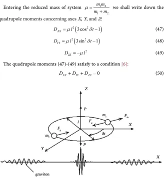
(46)

4. Gravitational Radiation of Double Stars

Let’s find the general energy flux of a gravitational radiation from the two bodies mass m1 and m2 the distance between which is equal l, moving on circular

orbits with frequency of rotation

δ

around of the common mass center, Figure 1. Such system is characteristic for double stars.

As well as everyone symmetric tensor the tensor Dik can be reduced in the

main axes.

Entering the reduced mass of system 1 2

1 2

m m m m µ =

+ we shall write down the

quadrupole moments concerning axes X, Y, and Z:

(

)

2 _3cos2 ₁ XX

D =µl δt− (47)

(

)

2 _3sin2 ₁ YY

D =µl δt− (48)

2 ZZ

D = −µl ₍₄₉₎

The quadrupole moments (47)-(49) satisfy to a condition [6]:

0

XX YY ZZ

[image:9.595.210.539.337.697.2]

D +D +D = ₍₅₀₎

(10)

According to the Formula (46) it is necessary to summarize the peak values of squares of third derivative on time from the quadrupole moments. It is con-nected by that in the Formula (33) the peak values of metric tensor hik are

used. Carrying out simple transformations we find:

(

)

2 2 2 2

3 3 3 3

,

2

2 3 2 4 6

2 12 288

ik XX YY ZZ

i k

D D D D

t t t t

l l

µ δ µ δ

∂  ₌∂  ₊∂  ₊∂ 

 _∂   _∂   _∂   _∂ 

     

 

= =

∑

(51)

The derivative from the quadrupole moment DZZ is equal to zero since it

does not depend on time.

Substituting (51) in (46) we find:

2 4 6 1 2 5

1 2

d 32

d 5

m m

E k _l

t c m m δ

 

− = _ _

+

  (52)

Let’s note that the gravitational radiation energy flux

2 4 6 1 2 5

1 2

1 d 16

2 d 5

m m

E k

P l

t c m m δ

 

= = _ _

+

  goes in both directions along axis Z [11],

Figure 1.

The Formula (52) is frequently written in the other kind [12]. Using equiva-lence of gravitational and inert masses, and hence the forces Fg=Fin, Figure 1,

we receive

(

)

2 3

1 2

k m m+ =

δ

l . Substituting the frequency

δ

in (52) we find:

(

) (

2

)

4

1 2 1 2

5 5

d 32

d 5

m m m m

E k

t c l

+

− = ₍₅₃₎

Formulas (52) and (53) have absolutely classical (not quantum) character. Outside a radiator of gravitational radiation the energy-impulse tensor

0

ik

T = _{. In this case the Equation (32) will be transformed to a kind:}

2 2

1 ₀

ik ik

h h

X Xα α c t

∂ ∂

− =

∂ ∂ ∂ (54)

The Equation (45) is the wave equation reflecting a propagation of the gravi-tational waves in empty space. Taking into account the gauge condition (30) and the Equation (54) by analogy to electromagnetic waves is possible to draw a con-clusion that gravitational waves are the cross-section waves propagating with a light velocity c.

The solution of the Equation (54) can be written down as [12]:

(

)

cos

ik ik

h =ae rX−δt (55)

where a there is an amplitude of a wave,

δ

-a frequency of gravitational waves,

r-a wave vector in a direction of a wave propagation. The value eik there is a

unit polarization tensor, obeying the conditions:

ik ki

e =e , eii =0, k ei ik=0, e eik ik=1 (56)

(11)

has essentially tensor character.

The third condition (56) is a condition of the gravitational waves cross-section.

5. Quantization of Gravitational Waves

At first point of view the quantization of a gravitational field can be carried out on analogies to a standard method of an electromagnetic field quantization, in particular, by a method of secondary quantization. Really, the equations of an electromagnetic wave include the wave equation and gauge equation. Similarly, the equation of a gravitational wave (54) is accompanied by the gauge Equation (27) which for a weak gravitational field passes in Lorentz’s gauge (30) identical to one gauges used in electrodynamics.

Therefore the gravitational field is a version of gauge fields [13].

However, for a gravitational field the situation is complicated two problems. First, the physical mechanism of reflection of gravitational waves from physical structures is not clear. Second, it is not known whether origination, and how of standing gravitational waves is possible.

5.1. Action of the Systems Gravitational Field-Particle

Both these unresolved problems now do application of a standard method for quantization of gravitational waves problematic.

Quantization of electromagnetic waves was carried out by quantization of the volumetric density of action in space of the generalized coordinates:

(

)

d d d d

s=

_∫

l t=

_∫

T U t− =

_∫

T t−

_∫

U t (57) where l T U= − there is total Lagrangian of a system a photon-particle and their interaction [14].

Let’s consider Lagrangian l of a systems a gravitational field-particle. Lagran-gian of this system looks like:

(

)

2

(

)

0 g g

l T U= − = ρ ρ− c − −g ρϕ −l −g (58)

where

(

)

2

0

T=

ρ ρ

− c −g there is the volumetric density of a kinetic energy of a particle in a gravitational field, U=

(

ρϕg−lg

)

−g —volumetric density of a

potential energy of a particle in a field (energy of interaction of a particle and field) including Lagrangian of the field [6]:

4

16π

g с

l R

k

= − (59)

where R there is a scalar curvature of a space-time, g<0—the determinant of a metric tensor, −g—defines the dependence of an volume normalizing ele-ment on space curvature,

ρ

—mass density of a particle in a field, ρ0—mass

density of a rest particle, ϕg—gravitational potential of a field.

Lagrangian to the Lagrange’s equation submits which looks like: d

d

l l

t

∂ ₌ ∂ _∂  _∂

(12)

For the generalized velocity we use size: 2T

=

q (61)

In this case the known formula for volumetric density of energy [6] is correct:

2 2

l l l T

w l T T U T T U T U

T

T T

∂ ∂ ∂ ∂

= − = − + = − + = +

∂ ∂ ∂ ∂

q q 

 (62)

owing to l 1

T

∂ ₌ ∂ .

From Formulas (58) and (61) follows that kinetic and potential energy of a particle in a gravitational field are equal:

(

)

2

2 0

2

T =q = ρ ρ− c −g_,U =

(

ρϕ_g −l_g

)

−g₍₆₃₎

Thus both components of volumetric density of action depend on a body den-sity which creates curvature of a space-time.

Therefore in the Einstein’s Equation (17) the right part of the equation de-pendent on mass creating a gravitational field should be subject to quantization only. The time is not quantized value. Apparently are not quantized all parame-ters of a space-time (scalar curvature, metric tensor, Ricci’s tensor, etc.). To quantization can be subject to only energy-impulse tensor.

5.2. Graviton Energy and Quantum Gravitational Eikonal

The quantum of a gravitational field–a graviton arises far from massive bodies where there is no gravitational field of these bodies. It arises due to curving by graviton of the Riemann’s spaces. Therefore a graviton has mass. The graviton mass is equal:

2

E m

c

= ₍₆₄₎

where Е there is a graviton energy, c—a light velocity.

Trace Т an energy-impulse tensor in Einstein’s equation is connected to scalar curvature of space-time R a ratio (20).

We use a sign plus in the Formula (20), since sizes in the left and right parts of equality positive. A sign minus is necessary to use in Lobachevski’s space to which Einstein’s equation it is applicable as absolutely general law of the nature.

If the graviton is propagated in a direction of an axis X1 the diagonal

com-ponents of a metric tensor owing to the cross-section of gravitational waves fol-lowing: h11=0, h22= −h33 [11]. The same ratio of components should be

ac-cording to (32) in the energy-impulse tensor of a graviton (18). Therefore a trace of a graviton energy-impulse tensor is equal

2 00 _Vm _VE

T T= = c =

(13)

8π

V k E R

c

= (65)

Action of a gravitational field is equal: dVd

g

S=

_∫

l t (66)

Lagrangian of a gravitational field it is equal [6]:

4

16π

g с

l R

k

= − (67)

Substituting (67) in (66) and assuming approximately constancy of scalar curvature in area of a graviton we shall find:

4

dVd V

16π

g с

S l t Rt C

k

=

_∫

= − + (68)

where C there is a constant of integration which can depend from X1.

Substituting (65) in (68) we have: 1 2

S= − Et C+ ₍₆₉₎

Further to similarly electromagnetic field, see (10), we shall enter into consid-eration concept of a quantum gravitational eikonal S=φ where



there is Planck’s reduced constant, φ=rX1−ωt—its phase, r—wave number of a

gra-viton, ω_{—its own frequency. We assume function of the quantum gravitational}

eikonal S X t

(

1,

)

approximately linear in a weak gravitational field [6][15]. We

shall note equivalence of quantum gravitational eikonal and actions of system a gravitational field—particle. Both sizes submit to a principle of a minimum (to Maupertuis’ principle for action or Fermat’s for eikonal) [6].

Let’s equate a quantum gravitational eikonal and action:

(

1

)

1₂

S=_φ=_ rX −ωt = − Et C+ ₍₇₀₎

From the Formula (70) follows that graviton energy is equal:

2

E= _

ω

₍₇₁₎

and size C=2rX1. The spin of graviton it is

±

2 

.

Energy of a relativistic mass particle is equal 2 2 2 4 0

E= p c +m c . Therefore, the Formula (71) allows to assume that as against an ordinary particle the gravi-ton rest mass is equal to zero m0=0, and the impulse of the graviton is equal

2 ₂

E

p r

c c

ω = =  = _ _.

Having substituted (71) in (64) we find 2 2

2 E m

c c

ω

= =  _{hence the mass of a}

graviton is proportional to its frequency. If for a graviton (by analogy to a pho-ton) the rule of “red displacement” operates then at removal from massive bo-dies the graviton frequency, and hence its mass should decrease down to disap-pearance of the graviton (gravitonic darkness1_{). At approach a graviton to the}

1_{It is possible that in the Universe there are the vivid individuals seeing with the help of gravitons as}

(14)

massive bodies the graviton frequency and its mass should increase.

If to accept for example the frequency of background thermal gravitational radiation _ω₌_{1.26 10 s}_× 12 −1 _[11]_{then graviton energy is}

15

2 2.66 10 erg 0.00166 eV

E₌ _ω₌ _× − ₌ _.

A graviton mass (64) of the background thermal gravitational radiations

26

2.96 10 g

m₌ _× − _.

Propagation of a graviton occurs in a direction of a normal to constant eikonal surface. Thus we have average radius of curvature of a constant eikonal surface (curvature of the Riemann’s spaces) in the given approximation (a weak gravita-tional field) are much greater of a graviton wave lengths λ 2πc

ω

= _[15]_.

5.3. The Quantum Form of an Energy-Impulse Tensor

Before to pass to the gravitational waves quantization we shall be solve one task. We shall find a gravitational field created any gas in space.

Let the size K k k= 1 2 is the Gaussian curvature of a 3-dimensional surface,

and 1 1

1

k =_ς _and ₂

2

1

k =_ς _{there are curvature in mutually perpendicular direc}

tions, ς1 and

ς

2-radiuses of curvature in these directions. Scalar curvature R

is connected with Gaussian curvature a simple ratio 1

2R K= [6].

Hence the Equation (20) can be transformed to a kind:

(

00 11 22 33

)

4 1 2

2 8π_{k T T T T}

c ς ς

− = + + + ₍₇₂₎

If a body creating a gravitational field is a gas, T11=T22=T33=P there is

pressure in gas, a size 2

00

T =ρc _,

ρ

_{-a gas density. Neglecting pressure in gas in}

comparison with a mass component 2

00

T =ρc , we have:

00 4 2 1 2

1 4πk_T 4πk

c c

ρ ς ς

− = = ₍₇₃₎

Assuming ς1=ς2 we shall find:

2 2 1

1 4πk c

ρ ς

− = ₍₇₄₎

Using a constant 27

2

4πk _{0.93 10 cm g}

c

−

= × _{and accepting gas density, for}

ex-ample, according to air density at a surface of the Earth _ρ₌_{1.3 10 g cm}_× −3 3_{, we}

find 2 30 2

1 2

4πk _{1.21 10 1 cm}

c

ρ

ς −

− = = × . Hence the radius of space curvature is

equal 15 10

1 1

1 0.91 10 cm 0.91 10 km

k

ς = = × = × _.

In calculation for reception of numerical values it was necessary to use the module of a square of curvature. There is an opportunity that space-time is a

pseudosphere of Lobachevski’s for which 2

1

K= −_ς _{. But we do not examine this}

(15)

them to compare any physical property of space-time.

We shall consider the energy-impulse tensor (18) in more detail. Into the energy-impulse tensor enters as making the stresses tensor:

11 12 13 21 22 23 31 32 33

X XY XZ

ik YX Y YZ

ZX ZY Z

T T T

σ

τ

σ

τ

σ

τ

σ

   

   

=_ _{ }= _

 

  _ _

 

(75)

where T T T11, 22, 33 there are normal stresses, other components σ =ik Tik for

i k≠ -tangential stresses. A component 2

00

T =ρc -volumetric density of energy,

10, 20, 30

Т Т Т -components of the impulse density multiplied on light velocity c,

01, 02, 03

Т Т Т -components of the energy flux density divided on c.

In a basis of the further research we shall assume absence of a stresses state birth of empty space owing to its possible curvature.

In [17] it has been shown that in a fluid and gas there is an uncertainty of a sign on tangential stresses. Moreover the stresses tensor only approximately de-scribes a stressed state of a fluid and gas. In a fluid and gas the stresses tensor is absent. For calculation of a fluid or gas flux it is necessary to use the vector for-mula connecting force dF and velocity

V

as [17]:

dF =ηdS×rotV (76) where dS there is area of contacting layers in a fluid or gas, η_{-viscosity tensor}

of the second rank, which diagonal components there are molecular viscosity, not diagonal components-turbulent viscosity.

If a flux of fluid or gas occurs for example in a direction axes X the directions of vectors in the Formula (76) are shown on Figure 2.

For our purposes in the Formula (76) using cyclic frequency of a medium

ro-tation 1 rot

2

=

ω V [18] it is convenient to write down as:

dF =2 dη S×ω (77) The scalar variant of the Formula (77) looks like:

(

) (

)

{

(

)

}

d d d

2 d d d d d d

X Y Z

Y Z Z Y Z X X Z X Y Y X

F F F

S S S S S S

η

ω

+ +

= − + − + −

i j k

i j k (78)

[image:15.595.283.461.595.707.2]

where i, j, k there are in this case unit vectors of 3-dimensional space. Assuming space homogeneous we use a scalar variant viscosity tensor

η

.

(16)

At use of the Formula (76) the uncertainty of the tangential stresses sign and some other problems connected with stresses tensor [17] on which we shall not stop disappear.

We shall write down the energy-impulse tensor (18) in the following kind:

2

01 02 03

3

1 2

10

1 1 1

3

1 2

20

2 2 2

3

1 2

30

3 3 3

d

d d

d d d

d

d d

d d d

d

d d

d d d

ik

с T T T

F

F F

T

S S S

T _T F F F

S S S

F

F F

T

S S S

ρ           =             (79)

where transition to digital indexes is carried out. Taking into account (78), we have:

(

)

(

)

(

)

(

)

(

)

(

)

(

)

(

)

(

)

2

01 02 03

2 3 3 2 3 1 1 3 1 2 2 1 10

1 1 1

2 3 3 2 3 1 1 3 1 2 2 1 20

2 2 2

2 3 3 2 3 1 1 3 1 2 2 1 30

3 3 3

2 d d 2 d d 2 d d

d d d

2 d d 2 d d 2 d d

d d d

2 d d 2 d d 2 d d

d d d

ik

с T T T

S S S S S S

T

S S S

T S S S S S S

T

S S S

S S S S S S

T

S S S

ρ

η ω ω η ω ω η ω ω

    − − −         = − − −      ₋ ₋ ₋        (80)

The tensor (80) is an energy-impulse tensor creating a curvature of a space-time. For quantization of the energy-impulse tensor first of all the size

η

should be expressed through the Planck’s sizes: Planck’s length

1 2 3 k c      

 _{, Planck’s}

time 1 2 5 k c      

 _{and Planck’s mass} c 12

k

     

 _{. Instead of size}

_η

_{we use it Planck’s}

value η=_V where V there is normalizing volume. Besides there are no reasons

to assume the areas in (80) various therefore shall accept dS1=dS2=dS3. In this

case the tensor (80) it will be transformed to a kind:

(

)

(

)

(

)

(

)

(

)

(

)

(

)

(

)

(

)

2

01 02 03 3 2 1 3 2 1 10

3 2 1 3 2 1 20

3 2 1 3 2 1 30

2 2 2

V V V

2 2 2

V V V

2 2 2

V V V

ik

с T T T

T T

T

T ρ

ω ω ω ω ω ω

    − − −       =_ ₋ ₋ ₋ _     − − −                (81)

Let’s consider for example the energy-impulse tensor for propagation of gra-vitational radiation to a direction of axis X1. Gravitational waves are

cross-section hence the vector of frequency is directed along an axis X1. In this

(17)

01 02 03

1 1 10 1 1 20 1 1 30 2 2 0 V V 2 2 0 V V 2 2 0 V V ik

с T T T

T T T T ρ ω ω ω ω ω ω      −    =  ₋       ₋            (82)

Asymmetry of the energy-impulse tensor Tik is connected with basic refusal

from use symmetric stress tensor [17].

In the tensor of energy-impulse the components 2 1

V

ω _ε

±  = ± _{enter which}

characterize volumetric density of energy of gravitational radiation quan-tum-graviton. Two signs of the spin are reflect two directions of polarization: (plus) a vector of cyclic frequency

ω

1 is directed along direction of a graviton

propagation and (minus) against direction of a graviton propagation.

In spite of the fact that we have entered the graviton energy in energy-impulse tensor it does not mean that tensor began to have quantum character. Further it is necessary to take into account ideas of the quantum mechanics matrix form and to add at least to tensor components with graviton energy a factor

(

1 1

)

exp_i S =_ expi rX −ωt

  [19] where S=φ is a quantum of gravitational

eikonal (70), φ=rX1−ω1t—its phase. We assume function of a gravitational

eikonal quantum S X t

(

1,

)

approximately linear in a weak gravitational field.

In the matrix form of quantum mechanics

ω

1 carries the name of spectral

frequency and characterizes transition of system from one quantum state in another. The factor exp_i S_

  characterizes transition of a gravitational field

quantum (graviton) on quantum states in a space-time. We shall note that at record of matrixes in the matrix form of quantum mechanics the exponential factors at a component of matrix frequently omit [19]. Thus the energy-impulse tensor will receive a kind:

(

)

(

)

2

01 02 03

10

20

30

2

01 02 03

1 1

10 1 1 1 1

1

20 1 1

0 exp exp

2 2

0 exp exp

V V

2

0 exp

V

ik

с T T T

i i

T S S

T _i _i

T S S

i i

T S S

с T T T

T i rX t i rX t

T i rX

ρ

ε ε

ρ

ω _ω ω _ω

ω _ω          ₋       _ _ _ _   =_ _ _ _ __ −      _ _ _ _      ₋        _ _ _ _   − − − = −         

₍

₎

₍

₎

(

)

(

)

1 1 1 1 1

30 1 1 1 1

2 _exp

V

2 2

0 exp exp

V V

t i rX t

T i rX t i rX t

ω _ω

ω _ω ω _ω

(18)

The energy-impulse tensor (83) has quantum character.

6. The Graviton Equation

For a finding of the graviton equation we shall substitute an energy-impulse tensor (83) in Einstein’s equation as (21). The tensor energy-impulse trace (83) looks like _T₌_ρ_c2_{. Hence the Equation (21)-the graviton equation will be}

transformed to a kind:

2 4

8π 1

2

ik k ik ik

R T g с

c ρ

 

= _ − _

  (84)

Let’s consider the graviton equation in almost flat space at absence of a mass component in energy-impulse tensor (84) i.e. at _T₌_ρ_c2₌₀_{. The gravitons}

practically do not bend space-time. Therefore it is possible to use the Formula (32):

The graviton radiation cross-section therefore all components in the Equation (32) with indexes 1 at the propagation of graviton in direction Х1 are

ex-cluded. Tensor components hik remain only: h23 and h22= −h33 [11]. We

shall notice also that in the energy-impulse tensor (76) T22= −T33.

For a component h23 the Equation (32) looks like:

(

)

2 2

23 23

1

2 2 2 4

1

1 16π 2 _exp

V

h h k _{i rX} _t

X c t c

ω _ω

∂ ∂

− = − −

∂ ∂

 ₍₈₅₎

For component h22 a sign in the right part of the equation is positive. The

index 1 at frequency is omitted.

Therefore designating χ =hikV where ik=22, 23, 33 we shall find:

(

)

2 2

1

2 2 2 4

1

1 32πk _exp_{i rX} _t

X c t c

χ χ ω _ω

∂ ∂

− = ± −

∂ ∂

 ₍₈₆₎

The factor before an exponent in the right part (86) is proportional to the double scalar curvature of space-time due to presence graviton, (65)

4 4

8π 8π 2

V V

k E k

R

c c

ω

= =  . This factor is extremely small

74 4

32πk _{0.87 10 cm s}

c

−

= × ⋅

 _{that specifies almost flat space-time.}

The Equation (86) describes a gravitational wave and graviton propagating from left to right therefore the general solution of the Equation (86) we shall search as:

(

)

( )

1 1 1 2 2 exp 1

С f rX t C f t irX

χ= −δ + ₍₈₇₎

where C1 and C2 there are constants, f rX1

(

1−δt

)

and f t2

( )

-any

func-tions,

δ

-gravitational wave frequency connected with a velocity of its propagation r

c

δ

= _{. Frequency}

δ

_{is not equal to own graviton frequency}ω_{. The}

(19)

(

)

2 2

1 2 2 2

1

1 _exp_{i rX} _t

X c t

χ χ _γω _ω

∂ ₋ ∂ _{= ±} ₋

∂ ∂ (88)

where it is designated 32π₄k c

γ = -a constant.

The first term (87) satisfies to the Equation (88) without the right part. Therefore after substitution we shall find:

(

)

2 2

2

d _exp ₀

d

f _f с _{i t}

C t

γω

δ ω

+ ± − = ₍₈₉₎

The particular solution of the Equation (89) dependent on own graviton fre-quency ω we shall search as:

(

)

2 exp

f =A −i tω (90) Substituting (90) in (89) we shall find:

(

)

2

2 2

2 с

A C

γω

ω δ

= ±

− (91)

Hence according to (87) the solution of the Equation (88) looks like:

(

)

₍

2

₎

(

)

1 1 ₂ с ₂ exp 1

С f rX t γω i rX t

χ δ ω

ω δ

= − ± −

− (92)

Taking into account a designation χ =hikV where ik=22, 23, 33, and also

4

32πk c

γ = _{, and (55), (65) we shall find:}

(

)

₍

₎

(

)

(

)

₍

₎

(

)

1 ₂ ₂ ₂ 1

2

1 ₂ ₂ 1

32π

cos exp

V 2

cos exp

ik ik ik

ik ik

k e

h ae rX t i rX t

c Rc e

ae rX t i rX t

ω

δ ω

= − −

−

= − −

−

 



(93)

where eik there is a unit polarization tensor (56).

The top sign in (92) and (93) corresponds gravitational additive to the metric tensor h22, and the bottom sign to h23 and h33; the first term is responsible

for propagation of the gravitational wave the second term characterizes graviton. The size hik naturally does not depend on normalizing volume V.

7. Registration of Graviton

The kind of function (93) allows draw some conclusions concerning interrela-tion of a gravitainterrela-tional wave and graviton. Far from massive bodies a graviton as the quantum effect is practically imperceptible. It practically has not influence on registration of the gravitational waves.

However function (93) has interesting feature. At

ω δ

→

_i.e. at aspiration of a graviton frequency to the gravitational wave frequency additional components of the metric tensor hik aspire to infinity. The resonance of the graviton and

(20)

Let’s assume that two massive cosmic bodies (for example a double star, Fig-ure 1) rotate around of the common mass centre. This system radiates gravita-tional waves hik=aeikcos

(

rX1−δt

)

with constant frequency

δ

(55). If

gra-viton gets in area of such cosmic bodies its own frequency ω grows according to the formula similar (9) for photon. According to the Formula (93) growth of a graviton energy occurs much faster 2

ω

that specifies resonant pumping of energy of these massive bodies gravitational field (through gravitational radia-tion P, Figure 1) in a graviton. Graviton energy can considerably exceed energy of a gravitational wave and finally graviton can be registered. Probably for this purpose it is necessary to install the detector on massive bodies or near to them (on their planet or the artificial satellite). With the help of such detector it is possible to register abnormal splash in gravitation at graviton passage.

At distance from the bodies a graviton return the energy to a gravitational field of the bodies; its frequency falls (as red displacement in gravitation), Figure 1. Therefore energy of a gravitational field of the massive bodies as a whole does not change at flight near them of gravitons. We shall notice also that Riemann’s curvature of space-time is positive therefore in the considered effect the addi-tional components of matrix tensor h23 and h33 take part only. They

reso-nantly grow at flight of a graviton near the massive bodies.

8. Conclusions

On the basis of Einstein’s equation for gravitation the gravitational radiation of a double star is investigated. By refusal from a stresses tensor into energy-impulse tensor, and replacement corresponding a component in power sizes also intro-ductions of a gravitational eikonal, the quantum quantization of gravitational radiation is lead.

The solution of the quantum equation of Einstein in the certain direction shows that this solution represents the sum of two composed, first of which cha-racterizes gravitational waves, and the second-graviton.

At approach of the gravitons to a double star there is a resonant pumping of the gravitational field energy through gravitational radiation to gravitons. It al-lows registering the gravitons. At distance of the gravitons from a double star their energy comes back in a gravitational field of the stars. Frequency of the gravitons decreases as red displacement for gravitation. Therefore as a whole the gravitons do not influence on a gravitational field of stars.

Conflicts of Interest

The authors declare no conflicts of interest regarding the publication of this pa-per.

References

[1] Bronstein, M.P. (1936) Quantization of Gravitational Waves. Moscow. Journal of Experimental and Theoretical Physics, No. 6, 195-236.

(21)

https://doi.org/10.1103/PhysRev.97.511

[3] Kiefer, C. (2004) Quantum Gravity. Oxford University Press, New York, 308. [4] Rubakov, V.A. and Tinyakov, P.G. (2008) Infrared-Modified Gravities and Massive

Gravitons. Uspekhi Fizicheskikh Nauk, 178, 785-822.

[5] Corda, C. (2009) Interferometric Detection of Gravitational Waves: The Definitive Test for General Relativity. International Journal of Modern Physics D, 18, 2275-2282. https://doi.org/10.1142/S0218271809015904

[6] Landau, L.D. and Lifshits, E.M. (1967) Theory of Field. Science, Moscow, 460. [7] Kaluza T. (1979) To Problem of Physics Unity, the Collection: Albert Einstein and

the Theory of Gravitation. Science,Moscow, 529-534.

[8] Pardo, K., Fishbach, M., Holz, D.E. and Spergel, D.N. (2018) Limits on the Number Spacetime Dimensions from GW170817. arXiv:1801.08160v1.

[9] Faddeev, L.D. (1998) Mathematical Physics. The Encyclopedia. In: Big Russian en-cyclopedia, Under Edit, Scientific Publishing House, Moscow, 153.

[10] Levich, V.G. (1962) Theoretic Physics Course. V. 1. FIZMATGIS, Moscow, 696. [11] Zeldovich, J.B. and Novikov, I.D. (1971) The Theory of Gravitation and Evolution

of Stars. Science,Moscow, 484.

[12] Peters, P.C. and Mathews, J. (1963) Gravitational Radiation from Point Masses in a Keplerian Orbit. Physical Review, 131, 435-440.

https://doi.org/10.1103/PhysRev.131.435

[13] Konopleva, N.P. and Popov V.N. (2000) Gauge Fields. Editorial URSS, Moscow, 272.

[14] Fradkin, E.S. (1965) The Method of Green’s Function in the Theory of the Quan-tum Fields and QuanQuan-tum Statistics, Moscow, Works FIAN. Science, 29, 7-138. [15] Levich, V.G., Vdovin, J.A. and Mjamlin, V.A. (1962) Theoretic Physics Course. V. 2.

FIZMATGIS, Moscow, 820.

[16] Bakelman, I.J. (1967) High Geometry. Education, Moscow, 349.

[17] Volobuev, A.N. (2012) Basis of Nonsymmetrical Hydromechanics. Nova Science Publishers, Inc., New York, 198.

[18] Schlichting, H. (1974) The Boundary Layer Theory. Science, Moscow, 63.