Comparative study of the mechanical behavior of the
superior thoracic artery and abdominal arteries using the
finite elements method
Kadri Salim, Bouchelaghem Abdelaziz Mahmoud, Bendjeddou Walid
Laboratory of Industrial Méchanic, University of Badji Mokhtar, Annaba, Algeria Email: [email protected]
Received 23 May 2011; revised 20 August 2011; accepted 19 December 2011
ABSTRACT
The human body has been the subject of thorough researches—not only from medical perspective but from a technical one as well—are very rich, amongst them we find blood circulation system comprising: the heart, the arteries and the veins. The overriding role of these researches is to explain some cardiovascular pathology and provide an aid tool for the endopro- thesis positioning in blood vessels while treating them. In this study we have developed a digital pattern us- ing the common (engineering technique of the) finite element method (FEM) to simulate the mechanical be- havior of the thoracic aorta and the abdominal aorta below the kidney under blood pressure effect. This pattern calculates the displacements, the stresses (con- straints) and the deformations of the two arteries’ walls enabling us to know their experimentally determined mechanical and geometric properties. This pattern could be applied to detect the aneurysm and dissection phenomena.
Keywords:Biomechanics; Finite-Element; Modeling;
Thoracic Aorta; Deformation (Strain) of the Arteries
1. INTRODUCTION
The mechanical behavior of the thoracic aorta is linked to the blood pressure (artery pressure) [1] where the pul- sating feature triggers dilatations and deformations of the wall which is constituted of three coats (layers) (the tu- nica intima, the tunica media and the tunica adventitia). This dilatation may multiply the risk of developing some pathology such as: the aneurysm and the dissection [2, 3].
In fact, the blood flows with a diastolic pressure (mini- mum pressure) then this latter increases to attain a systo- lic pressure (maximum blood pressure), the artery wall is then expanded owing to a radial traverse.
Due to the wall’s weak elasticity (advanced age) and the alternating pressure affecting this wall per se, this could trigger a aneurysm thoracic which is a very critical phenomenon because it doesn’t deform only the aorta but other adjacent organs as well if the dilatation is very severe. Besides it also alters the pulse wave’s value which causes a rupture (break) within another artery or a delay in blood distribution [4,5].
What’s more, the dissection is also a serious pheno- menon since it is tightly linked to the rupture of the arte- rial layer depending on its length; the latter could trigger the above mentioned phenomena on the other layers. In order to simulate the mechanical behavior of the thoracic aorta under blood pressure effect and make similarities with the abdominal aorta below the kidney—very known for specialists by its pathological phenomena—a pattern based on the finite element method has been adjusted. While situating ourselves in the small-deformation the- ory and considering the isotropic materials, the compre- ssible of E Young’s modulus and Poisson coeffi- cient [4], this pattern allows for calculating the displace- ments, the constraints and the deformations rates in the plan based on the mechanical properties of the thoracic aorta. Lots of researches had been carried out over the past several years in the arteriesmechanical properties field,Wang, J. J. Parker, K. H, have calculated the Young’s modulus in addition to geometries of 55 arteries in the human body [6].
2. BASIC EQUATIONS
Considering the arteries as a cylinder of an infinite length with an internal radius R1 and external radius R2 within
which blood circulates at Pint pressure. Under blood
pressure effect, the aorta’s wall undergoes radial dis- placement Ur and radial deformation rates εrr and angular εθθ which are given respectively bellow [4,5]:
d d r rr U r
r U
r
(2)
and
0 r zz z rz
Applying Hooke’s relation we can readily obtain the constraints rr, , zz:
2
ij ij kk ij
(3) In order to obtain the radial displacement function Ur we apply Navier-Lamé relation:
2
grad divU
rot rotU
f 0 (4) with f = 0 (gravity forces are considered negligible).In order to apply the finite element method we per- form a shift from cylindrical coordinates system to Car- tesian coordinates using:
cos sin x r y r z z
[image:2.595.310.539.84.194.2]In this case, the displacement becomes bi-dimensional (U, V) as well as the deformations and constraints (see
Figure 1) [7].
Problem data: geometries and mechanical properties of two arteries are given in the Table 1.
3. DIGITAL RESOLUTION
The finite element method consists in dividing the geo- metry into many elements then monitor element geome- try alterations in a thorough manner. These stages could be summarized as follow [8]:
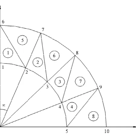
Step 1: mesh sizing: it is about putting nodes in the
geometry, and then numbering every and each node which allows the automatic determination of the triangular ele- ment associated with three nodes (Figure 2).
Identify the coordinates of each node according to one parameter which is the number of nodes (internal and external of the aorta).
Find the connection between then nodes’ numbering from one hand and the elements from another. For symmetry reason we carry out the mesh sizing except for a quarter of a pipe and considering the condi- tions of the limits (setting against x & y).
Step 2: calculate the three nodal coordinates of each
element (N1, N2, N3) in accordance with the coordinates
of each node.
Calculate the surface of each element.
Step 3: work out the elementary stiffness matrix
Km iusing the following formula:
Kmi
BT D B vd (5) [image:2.595.311.536.209.437.2]Step 4: assemblage of the elementary stiffness matrix
Figure 1. Geometry of the thoracic aorta.
[image:2.595.309.537.485.596.2]Figure 2. Mesh sizing of the arterial wall.
Table 1. Geometrical and mechanical characteristics of two arteries.
Geometrical and mechanical
properties thoracic aorta abdominal aorta
Inner radius R1 in cm 1.12 0.665
Outer radius R2 in cm 1.23 0.74
Thickness in cm 0.11 0.075
Young’s modulus in Pa 0.4 × 10⁶ 0.4 × 10⁶
Poisson’s ν coefficient 0.3 0.3
Arterial pressure [1,5]: Pint (diastolic) = 58 mmHg; Pint (medium) = 85 mmHg; Pint (systolic) = 122 mmHg.
Kv
Km i (6) Assemblage of the force vectors.
F
f i (7) where i in our case is the force resulting from pres- sure Pint.f
Step 5: work out the displacement vector (U, V) using
Kv U F (8) Stage 6: calculate the deformation and the constraintin every and each element using the same system apply- ing the elasticity hypothesis.
4. RESULTS AND DISCUSSION
We have carried out our calculation following the same example of Figure 2i.e. 10 nodes (5 on the R1 arc and 5
on the R2 arc), referring to our example we have also 8
elements.
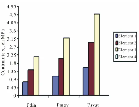
The curves bellow are displacement and constraint curves according to blood pressure Figure 3.
5. OBSERVATION
Constraints values of elements 4, 7 and 8 are negligible if compared to other constraints (see Figures 4 to 10).
[image:3.595.310.540.84.258.2]Thoracic Aorta Situation
[image:3.595.306.537.299.474.2]Figure 3. Constraints values σx applied on elements 1, 2, 3, 4 according to blood pressure.
[image:3.595.57.287.322.496.2]Figure 4. Constraints values σy applied on elements 1, 2, 3, 4 according to blood pressure.
[image:3.595.310.538.529.704.2]Figure 5. Constraints values σxapplied on elements 5, 6, 7, 8 according to blood pressure.
Figure 6. Constraints values σy applied on elements 5, 6, 7, 8 according to blood pressure.
Abdominal Aorta Situation
[image:3.595.58.288.536.706.2]Figure 8. Constraints values σy applied on elements 1, 2, 3, 4 according to blood pressure.
Figure 9. Constraints values σx applied on elements 5, 6, 7, 8 according to blood pressure.
Figure 10. Constraints values σyapplied on elements 5, 6, 7, 8 according to blood pressure.
These curves depict the increase of the applied con- straints as per x & y, this increase which is very much remarkable in the case of the internal wall (Tunica In- tima) is very high—compared to the thoracic aorta—on the abdominal aorta below the kidney, which explains the emergence of those two pathologies.
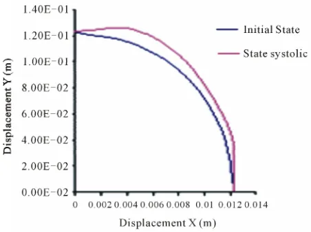
The bellow curves depict the position change of aorta walls under systolic pressure effect.
6. CONCLUSIONS
On the basis of the results of the present study, the nodes movement in the second arch, representing the outer layer of the thoracic aorta, rang from 6 to 10 mm, while those of the abdominal aorta range from 3 to 5 mm. These movements are not so important if one takes into account the respective geometry of the arteries, particularly their outer radius.
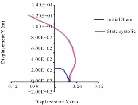
[image:4.595.308.534.351.522.2]The nodes movement in the first arch that represents the inner layer of the thoracic aorta, is about 10.8 cm, while those of the abdominal aorta is 11.2 cm (see Fig- ures 11 to 14).
Figure 11. Positions of the thoracic aorta internal wall nodes.
[image:4.595.59.288.525.704.2] [image:4.595.310.536.547.716.2]pressure does, but this increase is concentrated on the internal elements (see Figure 2). Hence, the requirement
of elastic nature intima firstly helps to prevent the break of this layer (dissection), and secondly to avoid the dis- placement of the three layers together at the same time which does not guarantee the return of one of the layers (aneurysm phenomenon).
Assuming that the aorta is rally circular, the change of that pace after the systolic pressure is enormous; there- fore this change affects the entire blood circulatory sys- tem, since it involves blood flow and distribution altera- tion.
[image:5.595.58.282.83.253.2]The results show that the risk of the above mentioned pathologies arising is greater for the abdominal aorta than for the thoracic one.
Figure 13. Positions of the abdominal aorta internal wall nodes.
REFERENCES
[1] Asmar, R. (2007) Préssion artérielle régulation et épidé- miologie, mesures et valeurs normales. Néphrologie & Thé- rapeutique, 21, 163-184.
http://www.sciencedirect.com/science/article/pii/S176972 5507001204
doi:10.1016/j.nephro.2007.03.008
[2] Roudant, R., Laurent, F. and Roques, X. (2002) Anévris- me de l’aorte thoracique. Edition Scientifiques et Médi- cales, 17, 11-500-A-10.
[3] Veyssier-Belot, C. (1998) Dissection aortique. La Revue de Médcine Interne, 4, 704-708.
doi:10.1016/S0248-8663(98)80704-2
[4] Wang, X., Wache, P., Navibakhsh, M., Lucius, M. and Stoltz, J.F. (1999) Simulation numérique tridimension- nelle de l’écoulement sanguin dans un anévrisme. Méca- nique Industrielle et Matériaux, 3, 71-74.
Figure 14. Positions of the abdominal aorta external wall
nodes. [5] Carli, F. and Martelli, M. (1999) Mechanical model of net
reinforced blood vessel. Advances in Engineering Soft-ware, 9, 673-681. doi:10.1016/j.jbiomech.2003.09.007 In terms of the inner layer, the displacements are con-
sidered very important to their in relation to geometry. [6] Wang, J.J. and Parker, K.H. (2004) Wave propagation in a model of the arterial circulation. Journal of Biomechanics, 13, 457-470.doi:10.1016/j.jbiomech.2003.09.007
We deduce that the arterial wall does not react in the same way as blood pressure: the inner layer or intima moves more significantly than the outer layer or adventi- tia. Unlike the movements of layers in the case of diastolic pressure and in the case of systolic pressure is high. This difference, applied alternately as in real life where the sys- tolic peak is oscillating, a break may appear in this area.
[7] Leslie, P., Gartner, J. and Hiatt, L. (1997) Atlas en couleur d’histologie. Pradel, Paris.
[8] Zienkiewicz, O.C. (2005) The finit element method for solid and structural mechanics. Elsevier Butterworth-Hei- nemann, Maryland Heights.
[image:5.595.58.286.291.465.2]NOMENCLATURE
B
D
: Deformation matrix : Matrix containing the elastic properties of the ma-terial (Hooke’s relationship)E: Young’s modulus
Km : Elementary stiffness matrix
Kv : Global stiffness matrix U : The displacement functionr
U : The radial displacement of the aorta
Pint: Blood pressure
N1, N2, N3: The coordinates of each nodal element
R1, R2: Inner and outer radius of the aorta
ij
: The constraints according to the coordinates (x, y) or (r, θ)
ij
: Deformation depending on the coordinates (x, y) or (r, θ)
,
: The Lame coefficients