A Practical Solution to the Small Sample Size Bias and Uncertainty Problems of Model Selection Criteria in Two Input Process Multiple Response Surface Methodology Datasets

ISSN Online: 2161-7198 ISSN Print: 2161-718X

DOI: 10.4236/ojs.2019.91010 Feb. 25, 2019 109 Open Journal of Statistics

A Practical Solution to the Small Sample Size

Bias and Uncertainty Problems of Model

Selection Criteria in Two-Input Process

Multiple Response Surface Methodology

Datasets

Domingo Pavolo, Delson Chikobvu

The University of the Free State, Bloemfontein, South Africa

Abstract

Multiple response surface methodology (MRSM) most often involves the analysis of small sample size datasets which have associated inherent statistic-al modeling problems. Firstly, classicstatistic-al model selection criteria in use are very inefficient with small sample size datasets. Secondly, classical model selection criteria have an acknowledged selection uncertainty problem. Finally, there is a credibility problem associated with modeling small sample sizes of the order of most MRSM datasets. This work focuses on determination of a solution to these identified problems. The small sample model selection uncertainty problem is analysed using sixteen model selection criteria and a typical two-input MRSM dataset. Selection of candidate models, for the responses in consideration, is done based on response surface conformity to expectation to deliberately avoid selection of models using the problematic classical model selection criteria. A set of permutations of combinations of response models with conforming response surfaces is determined. Each combination is op-timised and results are obtained using overlaying of data matrices. The permutation of results is then averaged to obtain credible results. Thus, a transparent multiple model approach is used to obtain the solution which gives some credibility to the small sample size results of the typical MRSM dataset. The conclusion is that, for a two-input process MRSM problem, conformity of response surfaces can be effectively used to select candidate models and thus the use of the problematic model selection criteria is avoidable.

How to cite this paper: Pavolo, D. and Chikobvu, D. (2019) A Practical Solution to the Small Sample Size Bias and Uncertainty Problems of Model Selection Criteria in Two-Input Process Multiple Response Surface Methodology Datasets. Open Jour-nal of Statistics, 9, 109-142.

https://doi.org/10.4236/ojs.2019.91010 Received: December 7, 2018

Accepted: February 22, 2019 Published: February 25, 2019 Copyright © 2019 by author(s) and Scientific Research Publishing Inc. This work is licensed under the Creative Commons Attribution International License (CC BY 4.0).

http://creativecommons.org/licenses/by/4.0/

DOI: 10.4236/ojs.2019.91010 110 Open Journal of Statistics

Keywords

Multiple Response Surface Methodology, All Possible Regressions, Model Selection Criteria, Data Matrices

1. Introduction and Literature Review

Multiple response surface methodology (MRSM) is when an industrial process with more than one response variable is investigated and studied through the analysis of reliably generated response models and corresponding response sur-faces at some region of operability. Processes with two inputs provide a special case of MRSM problems whose response surfaces can be constructed in three dimensions and therefore can be analysed for conformity.

Hill & Hunter [1] are credited with originally identifying the existence of MRSM in their review paper in response surface methodology. In their review of developments in response surface methodology research from 1966 to 1988, Myers et al. [2], conclude that most problems encountered in literature and practice are in fact MRSM problems as opposed to single response models (un-ivariate case). Khuri [3] single handedly wrote a full review of MRSM. Mukho-padhyay & Khuri [2] and Khuri [4] afforded sections of MRSM in their latest response surface methodology reviews.

Myers et al.[5] emphasise that MRSM should always include canonical and response surface analysis before optimisation. Khuri [3] [4] clearly argues that traditional response surface techniques that apply to single response models, in general, are not adequate to analyse multiple response problems. Khuri [3] and Mukhopadhyay & Khuri [2] emphasize the use of multivariate statistical me-thods in every stage of MRSM processes so that the responses are considered simultaneously in every aspect, especially where correlation exists between the responses. Figure 1 shows the MRSM contextual framework as developed from literature.

The first of three problems with industrial MRSM work is the uncertainty in-herent in the process of model selection (Wit et al., [7], Steel [8], Moral-Benito

[9]) and this worsens when sample sizes are small. Hjort and Claesken [10] state that the uncertainty associated with the model selection process can make the inference based on the final model to be seriously misleading. Danilove and Magnus [11] add that standard errors that are estimated under such circums-tances are known to underreport variability. This problem can be solved by avoiding the use of model selection criteria in the selection of best models from candidate models.

DOI: 10.4236/ojs.2019.91010 111 Open Journal of Statistics

The second problem concerns the small sample size bias problem of classical model selection criteria. MRSM is largely a regression modeling and model se-lection problem. Model sese-lection is done through model sese-lection criteria. Seg-houane and Bekara [12] state that the derivations of most model selection crite-ria like Mallow’s Cp [13], Akaike’s AIC [14] and Schwarz’s SBC [15] rely on asymptotic approximations which are not valid for small sample sizes. Most MRSM experimental datasets fall within the small sample size context. The use of such criteria for the small sample size context problems results in increased bias.

Attempts have been made to correct some of the classical model selection cri-teria for the small sample size context. Suguira [16] corrected the Akaike’s in-formation criterion (AIC) for small samples by making the assumption of a fi-nite true model and avoiding the asymptotic argument in his derivation of the corrected AIC (AICc). Hurvich and Tsai [17], after some simulation tests, con-firmed that AICc achieves dramatic reductions in bias in small sample sizes compared to AIC and even Schwarz’s SBC. They recommend its use in place of AIC for small sample size problems. McQuarrie and Tsai [18] corrected Hannan and Quinn [19]’s consistent criterion for small sample sizes to come up with the corrected HQ (HQc). Sawa [20] also did a small sample correction to Schwarz’s SBC to come out with BIC. Seghouane and Bekara [12] did a small sample cor-rection to their Kullback-Leibler symmetric divergence information criterion (KIC) to come up with corrected KIC (KICc). Literature is quite silent in the ap-plication of such research findings in MRSM. Both Myers et al.[5] and Khuri [4]

do complain on the lake of uptake of research findings by MRSM practitioners. The extent to which the small sample size bias problem has been solved by the small sample size correction efforts can be analysed using an MRSM dataset. In 1999 Pan [21] released his proposal of using bootstrapping for model selection with small samples. There are also proposals to look into model averaging (Yuang and Yang [22], Xie [23]).

In accordance with the information-theoretic approach, a “best model” for analysis of data depends on sample size as smaller effects can often only be re-vealed as sample sizes increase. The amount of information in large datasets greatly exceeds the information availed by small datasets.

The small sample size bias problem and the one of model selection uncertain-ty are related in that they all have to do with the use of model selection criteria in choosing the best model. If the use of model selection criteria is avoided for the use of an approach with more certainty, both problems will be solved.

DOI: 10.4236/ojs.2019.91010 112 Open Journal of Statistics

industrial examples used in Myers et al. [5] and [24] do not have experimental runs (n) > k * 40. This critical problem has not been dealt with in MRSM re-search studies so far. Khuri [4] does not even mention this problem in his pro-posals of areas of future research in MRSM. This problem is dealt with by using a solution methodology that has more rigour and transparency.

The three problems encountered by MRSM practitioners related to the small sample MRSM dataset sizes are shown in Figure 2.

This paper focuses on the problems encountered with the use of model selec-tion criteria in selecting best models with particular interest in MRSM. In other words, the focus is on obtaining the best result instead of the best models to use in optimization. In this way,

1) Sets of candidate models are selected based on conformity of response sur-faces for each response,

2) Permutations of response model combinations are made,

3) Simultaneous “optimisation” is performed of response model combina-tions, and

4) The best result is obtained even by averaging.

The use of conformity of response surfaces to select candidate models for op-timisation instead of model selection criteria is investigated in this paper. The use of conformity of response surfaces enables avoidance of model selection cri-teria and thus indirectly solves the model selection cricri-teria uncertainty problem. In the same manner, the avoidance of the use of model selection criteria in mod-el smod-election indirectly solves the worry of the small sample size bias problem. The selection of response candidate models based on their conformity of response surfaces enables the determination of candidate model combinations for opti-misation. The permutation of response model combinations converts to the permutation of results which can be averaged to obtain the best result. This mul-ti-model approach maintains the rigour required in model selection to ensure convincing and credible solutions for the small sample size problems in MRSM. The proposed MRSM theoretical framework of the current study is shown in

Figure 3.

DOI: 10.4236/ojs.2019.91010 113 Open Journal of Statistics Figure 3. Multiple response surface methodology theoretical framework.

The remainder of this paper is organized as follows. Section 2 introduces the typical small sample MRSM dataset, which will be subjected to analysis in this study. Section 3 analyses the typical small sample MRSM dataset with sixteen model selection criteria taken from literature exposing the selection uncertainty problem in MRSM small sample sizes. In Section 4, the MRSM small sample size problem is resolved by a multi-model approach and the results are analysed. Section 5 looks at the validation of the results in line with the original problem of obtaining cure times of rubber covered mining conveyor belts for a Southern African manufacturer. Section 6 discusses findings and Section 7 concludes and proposes direction of future research.

2. The Dataset

The MRSM experimental design and results used for the current study are shown in Table 1. The experimental design is a two-factor central composite de-sign [25] [26]. The experimental runs were done to determine the best cure times for different industrial and mining conveyor belt thicknesses for a South-ern African rubber covered mining conveyor belts manufacturing company. The two input parameters into the belt curing process are cure time (T) and rubber thickness (RT). The measured quality responses are adhesion of belt compo-nents (in N/mm) and hardness of cured rubber cover (in Shore A).

This dataset is chosen for use in this investigation because, in addition to be-ing a typical small sample MRSM dataset, two factor experiments produce re-sponse models that have rere-sponse surfaces that can be analysed. Where factors are more than two, it is difficult to construct response surfaces of models in three dimensions. So two factor processes are a special case of MRSM where it is possible to check response model fitness to data, prediction performance and analyse response surface model conformity to expectations before selection of “best” model for consideration in multi-objective optimisation. More complex problems require more complex ways to solve them.

3. All Possible Regressions Modeling

All possible regressions modeling is applied to the dataset in Table 1 to obtain thirty one (2p−1_{, where p is the total number of regressors) models for each of the}

two responses, that is, adhesion and hardness. ANNEXURE A shows the thirty one models of each response in detail.

4. The Model Selection Uncertainty

DOI: 10.4236/ojs.2019.91010 114 Open Journal of Statistics Table 1. Experimental design and averaged results from the MRSM experiment.

Run Random X1

(T = TIME) (RT = RUBBER THICKNESS) X2 Ave. Adhesion (N/mm) Ave. Hardness (˚shore A) 1 7 16 7.2 10.60 60 2 9 30 7.2 13.34 63 3 11 16 22.8 6.20 53 4 8 30 22.8 12.10 61 5 1 23 15 11.80 58 6 5 23 15 12.10 58 7 4 13 15 6.5 44 8 2 33 15 13.30 63 9 10 23 4 13.30 63 10 3 23 26 3.50 56 11 6 23 15 12.20 58 12 12 23 15 12.30 57 13 13 23 15 12.10 58

able to bring out the between-criteria uncertainty problem into the limelight. The thirty one all possible regressions response models which are generated from the results of the MRSM experiment are analysed using sixteen different model selection criteria. The sixteen model selection criteria are used to select the best model for adhesion and hardness between the thirty one all regression models. Ten of the sixteen model selection criteria are corrected for small sam-ple size inefficiency; three are not corrected and choose the best model fitting the MRSM dataset, while three choose the best model for prediction. The formulae and relevant details of the selection criteria are given in ANNEXURE B.

Model Selection Uncertainty 1: Model selection criteria do not necessarily agree on the best model

 Adhesion

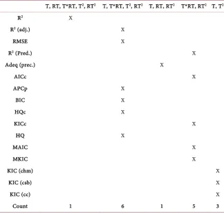
Table 2 shows the models chosen as best by each criterion. The model se-lected as best by each criterion is marked by X.

There are two adhesion response models with the most selections in Table 2: one with six, [T*RT, RT2_{], and the other with five, [T, T*RT, T}2_{, RT}2_{]. Another}

DOI: 10.4236/ojs.2019.91010 115 Open Journal of Statistics Table 2. Showing selection criteria and the selected adhesion “best” models.

T, RT, T*RT, T2_{, RT}2 _{T, T*RT, T}2_{, RT}2 _{T, RT, RT}2 _{T*RT, RT}2 _{T, T}2

R2 _X

R2 _{(adj.) X}

RMSE X

R2 _{(Pred.) X}

Adeq (prec.) X

AICc X

APCp X

BIC X

HQc X

KICc X

HQ X

MAIC X

MKIC X

KIC (chm) X

KIC (csb) X

KIC (cc) X

Count 1 6 1 5 3

 Hardness

The model selection uncertainty problem is again evident with hardness as shown in Table 3. One model, [T, RT, T*RT, T2_{, RT}2_{], is selected by eleven}

dif-ferent criteria whilst another two are selected for the remaining five times. Even the ten small sample size corrected criteria do not agree with five choosing the full model, three choosing [T, T2_{] and two [T, T}2_{, RT}2_{]. This uncertainty is}

cha-racteristic of the model selection process which selects one model as best.

Model Selection Uncertainty 2: Good fitness to data and/or good prediction performance does not imply conforming response surface

 _{Analysis of Response Surfaces}

Response surfaces for each of the thirty one models are obtained and analysed as to whether they conform to expectations. Data matrices are constructed to confirm.

Only four adhesion response models have conforming response surfaces which are: [T, RT, T*RT]; [T, RT, T*RT, T2_{]; [T, RT, T*RT, RT}2_{], and [T, RT,}

T*RT, T2_{, RT}2_{]. Only one hardness model has a conforming response surface}

which is [T, RT, T*RT, T2_{].The response surfaces are shown in ANNEXURE C.} Table 4 summarises the results of the analysis of response surfaces.

DOI: 10.4236/ojs.2019.91010 116 Open Journal of Statistics Table 3. Showing selection criteria and the selected hardness best model.

T, RT, T*RT, T2_{, RT}2 _{T, T}2_{, RT}2 _{T, T}2

R. Sq. X R. Sq. (adj.) X RMSE X

R. Sq. (Pred.) X Adeq. (prec.) X

AICc X APCp X BIC X HQc X KICc X

HQ X

MAIC X

MKIC X

KIC (chm) X

KIC (csb) X

KIC (cc) X

11 2 3

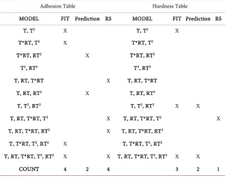
Table 4. Summarising model selection results split between fit to data, prediction and conforming Response Surface (RS).

Adhesion Table Hardness Table

MODEL FIT Prediction RS MODEL FIT Prediction RS T, T2 _{X T, T}2 _X

T*RT, T2 _{X T*RT, T}2

T*RT, RT2 _{X T*RT, RT}2

T2_{, RT}2 _T2_{, RT}2

T, RT, T*RT X T, RT, T*RT T, RT, RT2 _{X T, RT, RT}2

T, T2_{, RT}2 _{T, T}2_{, RT}2 _{X X}

T, RT, T*RT, T2 _{X T, RT, T*RT, T}2 _X

T, RT, T*RT, RT2 _{X T, RT, T*RT, RT}2

T, T*RT, T2_{, RT}2 _{X T, T*RT, T}2_{, RT}2

T, RT, T*RT, T2_{, RT}2 _{X X T, RT, T*RT, T}2_{, RT}2 _{X X}

DOI: 10.4236/ojs.2019.91010 117 Open Journal of Statistics

response surface at the same time. Best fit and/or best prediction does not ensure conforming response surface. This is the second uncertainty problem.

Model Selection Uncertainty 3: Good fitness to data does not necessarily imply good prediction performance

The other uncertainty problem is that a model with good fitness to data is not necessarily good at prediction performance. This is evident from the table. This is the third model selection uncertainty problem.

Model Selection Uncertainty 4: The uncertainty of positioning/ranking by the individual criteria

Figure 4 shows how each of the four adhesion models with conforming re-sponse surfaces is ranked by each selection criterion. The only hardness model with a conforming response surface that is selected as best fitting is the full mod-el which is smod-elected by R2 _only.

In addition to the uncertainty of selection as “best” model, as previously noted, there is also the uncertainty of positioning/ranking by the individual cri-teria. One cannot predict the positioning/ranking of models by the individual criteria.

The best selection position of the only hardness model with the conforming response surface is number three as seen in Figure 5. Seven model selection

Figure 4. Showing how the 4 adhesion models with conforming responses surfaces are ranked by different criteria.

DOI: 10.4236/ojs.2019.91010 118 Open Journal of Statistics

criteria put this model on position three in their rankings. However, the same response model is ranked twenty five by four other criteria. There is, therefore, no known formula to predict the ranking of the models with conforming re-sponse surfaces, as different selection criteria rank them differently. The only way that models with conforming response surfaces can be recognised is by in-specting response surfaces. This is now the fourth model selection uncertainty problem.

5. Effect of Correction of Model Selection Criteria

Twenty eight model selection criteria are used to select the best model and the frequency of selection per number of regressor variables (p) is determined. This is done for each of the response variables of adhesion and hardness.

Adhesion

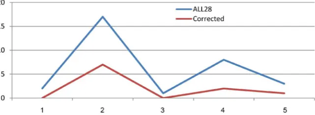
Table 5 is for the adhesion response. Row 2 of Table 5, titled “ALL 28”, summarises the findings. Row 3, titled “Corrected”, has the frequency details of the ten small sample size corrected criteria.

A visual picture of Table 6 is shown by Figure 6.

The mere fact that there is a selection for each p-value when all the twenty eight model selection criteria are used indicates model selection uncertainty.

Table 6 shows that when only the ten small sample size corrected criteria are considered, two facts emerge: 1) there is zero selections for the three regressor

Figure 6. Showing the model selection results per number of regressors (p) for the adhe-sion response.

Table 5. Summarising model selection results per number of regressors (p) for the adhe-sion response.

REGRESSORS (p) 1 2 3 4 5 ALL 28 2 17 1 8 3 Corrected 0 7 0 2 1

Table 6. Showing model selection results for pooled regressors before and after the me-dian for the adhesion response.

DOI: 10.4236/ojs.2019.91010 119 Open Journal of Statistics

position and the one position, and 2) there are seven selections to the left of three regressors (median term) and only three to the right.

Hardness

Table 7 is for the hardness response. Row 2 of Table 7, titled “ALL 28”, summarises the findings. Row 3, titled “Corrected”, has the frequency details of the ten small sample size corrected criteria.

Table 7 gives the following line graph shown in Figure 7.

Uncertainty in selection is obvious in both the adhesion and hardness cases where twenty eight model selection criteria are used and when only small sample size corrected criteria are used.

Table 8 again queries the principle of parsimony as the small sample size cor-rected criteria select no model with three regressors (median term) but select four models to the left hand and six models to the right hand of the median term. It appears the major achievement of small sample size correction is the zeroing of the middle term.

This could be posing a query to the achievement of parsimony in balancing bias (lack of fit) and penalty especially where small sample size corrected criteria is concerned as there could be over-correction which results in criteria selecting models with fewer regressors or underfitting in trying to correct small sample size inefficiency.

Figure 7. Showing the model selection results per number of regressors (p) for the adhe-sion response.

Table 7. Summarising model selection results per number of regressors (p) for the hard-ness response.

REGRESSORS (p) 1 2 3 4 5 ALL 28 1 5 2 4 16 Corrected 1 3 0 3 3

Table 8. Showing model selection results for pooled regressors before and after the me-dian for the hardness response.

DOI: 10.4236/ojs.2019.91010 120 Open Journal of Statistics

6. Optimisation

MRSM is based on the use of response surfaces of a selected combination of re-sponse models to simultaneously determine the region with the desired results. There being no certain method of using a classical model selection criterion to predict models with conforming response surfaces implies the simplest way to deal with the problems of model selection uncertainty and small sample size bias is to avoid choosing candidate “best” models with model selection criteria. In two-input MRSM processes this is possible as response surfaces can be used to select candidate models. Therefore, in this section the four possible results from the permutations of the four adhesion response surfaces and one hardness re-sponse surface are analysed. The four results are obtained by simultaneously solving the tabled four pairs of models. The mean square errors (MSE) of the conforming models are also determined.

6.1. The Permutations of Models with Conforming Response

Surfaces

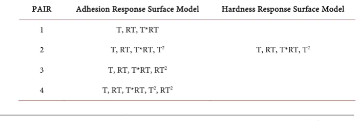
The permutations of adhesion-hardness response model pairs with conforming response surfaces is shown summarized in Table 9. The four pairs form the set of candidate pairs for optimisation or determination of desired results.

6.2. The Determination of Desired Results

The desired results are obtained by constructing data matrices for each response in a candidate pair using Microsoft Excel and overlaying them to determine the region where the two response models simultaneously achieve customer ex-pected results of adhesion ≥ 12 N/mm and hardness ≥ 60 ˚Shore A. The detailed process of determination of desired results for each combination is shown in ANNEXURE D. Pair 2 is used here as an example to demonstrate the process.

Pair 2: [T, RT, T*RT, T2_{] vs. [T, RT, T*RT, T}2_]

The response surfaces and corresponding data matrices of Pair 2 are presented as an example. The data matrices are overlaid to obtain the desired region from which results of cure time per rubber thickness are obtained. The boxed figure 9 in the data matrix in Table 10 is obtained by setting a time of 22 minutes for a belt with rubber thickness 20 mm.

Table 9. Showing the four pairs of four adhesion models and the one hardness model with conforming response surfaces.

PAIR Adhesion Response Surface Model Hardness Response Surface Model 1 T, RT, T*RT

2 T, RT, T*RT, T2 _{T, RT, T*RT, T}2

3 T, RT, T*RT, RT2

DOI: 10.4236/ojs.2019.91010 121 Open Journal of Statistics Table 10. Showing the data matrix of the adhesion model [T, RT, T*RT, T2_].

CT 21 22 23 24 25 26 27 28 29 30 RT

20 9 9 9 10 10 11 11 11 11 12 19 9 9 10 10 11 11 11 11 12 12 18 9 10 10 10 11 11 11 12 12 12 17 10 10 10 11 11 11 12 12 12 12 16 10 10 11 11 11 12 12 12 12 13 15 10 11 11 11 12 12 12 12 13 13 14 11 11 11 12 12 12 12 13 13 13 13 11 11 12 12 12 12 13 13 13 13 12 11 12 12 12 13 13 13 13 13 13 11 12 12 12 13 13 13 13 13 14 14 10 12 12 13 13 13 13 13 14 14 14 9 12 13 13 13 13 14 14 14 14 14 8 13 13 13 13 14 14 14 14 14 14 7 13 13 14 14 14 14 14 14 14 14

 _{Adhesion [T, RT, T*RT, T}2_{] Data Matrix}

The data matrix for the adhesion model [T, RT, T*RT, T2_{] if overlaid with a}

hardness model data matrix from a conforming response surface gives the de-sired region with optimum cure time per rubber thickness.

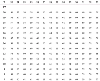
 Hardness [T, RT, T*RT, T2_{] Data Matrix}

The hardness data matrix of Table 11 for model [T, RT, T*RT, T2_{] is overlaid}

with the data matrix for the adhesion model [T, RT, T*RT, T2_{] to give the}

de-sired region with cure time per rubber thickness meeting customer expectations.

Table 12 shows the region in red in which both the adhesion and hardness are within the customer specified region of adhesion ≥ 12 N/mm and hardness ≥ 60 ˚Shore A.

Cure times per belt rubber thickness are selected to ensure customer expecta-tions are met and right levels of productivity maintained. The region in red has both adhesion and hardness results in levels acceptable to the customer expecta-tions. The boxed figures in the desired region indicate the cure time per belt rubber thickness combinations considered for work instructions.

6.3. MSE’s of Conforming Response Models

Mean Sum of Squares (MSE’s) for the models with conforming response surfaces are determined using Equation (9) for comparing of accuracy of response mod-els. The formula for MSE is given below for a sample size n.

(

)

1 ˆ

MSE

n i i i Y Y

n

= −

=

∑

DOI: 10.4236/ojs.2019.91010 122 Open Journal of Statistics Table 11. Showing the data matrix of the hardness model [T, RT, T*RT, T2_].

T 20 21 22 23 24 25 26 27 28 29 30 31 32 33 RT

20 56 57 58 59 59 60 60 60 60 60 60 60 60 59 19 56 57 58 59 59 60 60 60 61 60 60 60 60 59 18 57 58 58 59 60 60 60 60 61 60 60 60 59 59 17 57 58 59 59 60 60 60 61 61 60 60 60 59 59 16 57 58 59 59 60 60 60 61 61 60 60 60 59 59 15 57 58 59 60 60 60 61 61 61 60 60 60 59 58 14 58 59 59 60 60 60 61 61 61 60 60 60 59 58 13 58 59 59 60 60 61 61 61 61 60 60 60 59 58 12 58 59 60 60 60 61 61 61 61 60 60 59 59 58 11 59 59 60 60 61 61 61 61 61 60 60 59 59 58 10 59 60 60 60 61 61 61 61 61 60 60 59 59 58 9 59 60 60 61 61 61 61 61 61 60 60 59 58 58 8 59 60 60 61 61 61 61 61 61 60 60 59 58 57 7 60 60 61 61 61 61 61 61 61 60 60 59 58 57

Table 12. Showing the region of overlay with the wanted results.

_CT

RT 21 22 23 24 25 26 27 28 29 30

20 60

19 60 60

18 61 60 60

17 61 61 60 60

16 60 61 61 60 60

15 60 61 61 61 60 60

14 60 60 61 61 61 60 60

13 60 60 61 61 61 61 60 60

12 60 60 60 61 61 61 61 60 60

11 60 60 61 61 61 61 61 60 60

10 60 60 60 61 61 61 61 61 60 60

9 60 60 61 61 61 61 61 61 60 60

8 60 60 61 61 61 61 61 61 60 60

7 60 61 61 61 61 61 61 61 60 60

7. Results

DOI: 10.4236/ojs.2019.91010 123 Open Journal of Statistics

7.1. Tables of Rubber Thickness vs. Cure Time

Using overlaying of data matrices, tables of rubber thickness-cure time combi-nations are determined for the four pairs of models. The tables are shown as

Tables 13-16.

If all the result tables are averaged, a result equivalent to Table 14 and Table 15 is obtained. This result is both the median and mode of the tables and is therefore the best to adopt for use.

7.2. MSE’s of Models with Conforming Response Surfaces

Response model accuracy is checked by the size of the MSE. Table 17 shows the computed MSE values of models with conforming response surfaces.

The MSE values for adhesion models show that the full model, [T, RT, T*RT, T2_{, RT}2_{], has the best fit-to-data accuracy compared to the other three models}

with conforming response surfaces.

Table 13. Pair 1 [T, RT, T*RT] vs. [T, RT, T*RT, T2_].

Rubber Thickness (mm) 7 8 9 10 11 12 13 14 15 16 17 18 19 20 Cure Time (min.) 21 22 23 24 24 25 25 26 26 27 28 28 29 30

Table 14. Pair 2 [T, RT, T*RT, T2_{] vs. [T, RT, T*RT, T}2_].

Rubber Thickness (mm) 7 8 9 10 11 12 13 14 15 16 17 18 19 20 Cure Time (min.) 21 22 23 24 24 25 25 26 26 27 27 28 29 30

Table 15. Pair 3 [T, RT, T*RT, RT2_{] vs. [T, RT, T*RT, T}2_].

Rubber Thickness (mm) 7 8 9 10 11 12 13 14 15 16 17 18 19 20 Cure Time (min.) 21 22 23 24 24 25 25 26 26 27 27 28 29 30

Table 16. Pair 4 [T, RT, T*RT, T2_{, RT}2_{] vs. [T, RT, T*RT, T}2_].

Rubber Thickness (mm) 7 8 9 10 11 12 13 14 15 16 17 18 19 20 Cure Time (min.) 21 22 23 24 24 25 25 26 26 27 27 28 28 29

Table 17. Showing MSE results for adhesion and hardness.

ADHESION HARDNESS

MSE MSE

T, RT, T*RT 2.3441

T, RT, T*RT, T2 _{2.1777 T, RT, T*RT, T}2 _5.3806

T, RT, T*RT, RT2 _1.2789

DOI: 10.4236/ojs.2019.91010 124 Open Journal of Statistics

8. Validation

The results from the first seven conveyor belts to be run from the process, shown in Table 18, are compared with model forecasted results by a paired T-Test and the mean forecasted squared errors (MSFE) of response models are computed.

Validation by T-Tests

The first validation test proves that there is no significant statistical difference between the forecasted results and the results obtained from belts run from the normal belt production process. The results from the first seven conveyor belts to be run from the process are compared from model forecasted results using a paired T-Test as shown in Figure 8.

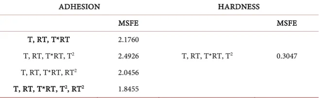
Validation by MSFE

In this section, validation of results is done by checking the effectiveness to obtain better or the same rubber thickness-cure time combinations as obtained in the first MRSM experiment.

(

)

1

SFE

n

i Fi

i Y Y

n

= −

=

∑

where Yi is ith the measured response, YFi is the ith forecasted response.

The MSFE values for adhesion models shown in Table 19 reveal that the full model, [T, RT, T*RT, T2_{, RT}2_{], has the best prediction accuracy compared to the}

Figure 8. Showing the paired T-Test results.

Table 18. Validation results.

# Thickness Rubber (mm)

Cure Time (min)

Actual Adhesion

(N/mm)

Predicted Adhesion (N/mm)

Adhesion Error (N/mm)

Actual

DOI: 10.4236/ojs.2019.91010 125 Open Journal of Statistics Table 19. Showing MSFE results for adhesion and hardness.

ADHESION HARDNESS

MSFE MSFE

T, RT, T*RT 2.1760

T, RT, T*RT, T2 _{2.4926 T, RT, T*RT, T}2 _0.3047

T, RT, T*RT, RT2 _2.0456

T, RT, T*RT, T2_{, RT}2 _1.8455

other three models with conforming response surfaces. The best combination of adhesion versus hardness models for the best accuracy results is therefore the pair: Pair 4 [T, RT, T*RT, T2_{, RT}2_{] vs. [T, RT, T*RT, T}2_].

Averaging all the results tables gives a table similar to Table 14 and Table 15. The table represented by Table 14 and Table 15 is therefore both the mean and mode of the permutation of results. This shows that it is a robust result. This re-sult would be the best to use in Work Instructions in this case.

9. Discussion

This section discusses the small sample size MRSM datasets problems of using classical model selection criteria to select “best” models for use in determining desired solutions and how they are solved.

The Small Sample Size Bias Problem

The small sample size model selection criteria bias problem is solved by avoiding the use of model selection criteria for selecting “best” models in this study. In fact where response surfaces can be used to select candidate models, classical model selection criteria become irrelevant with all their problems.

The Model Selection Uncertainty Problem

The model selection uncertainty problem is related to the use of classical model selection criteria for selecting best models. Even the use of small sample size corrected criteria is shown to have the problem of model selection uncer-tainty. It is difficult to predict a model with a conforming response surface with classical best model selection criteria whether small sample size corrected or not. MRSM depends a lot on the use of conforming response surfaces in simulta-neously determining the desired results. Research on design of experiments for MRSM should focus more on determining conforming response surfaces than just models with good fit to available data or prediction. The conformance of the response surface within the region of interest should be the focus of MRSM ex-perimental designing research.

Using Response Surfaces to Select Response Models

DOI: 10.4236/ojs.2019.91010 126 Open Journal of Statistics

The use of response surfaces to select conforming models is very possible with two-factor multiple regression models although it is not that easy with processes of more than two factors. However, whilst still dealing with two factor processes, selecting models based on conformity of response surfaces avoids use of classical model selection criteria in choosing the best models and hence the problems of model selection criteria uncertainty and small sample size datasets bias. In MRSM that is very important. Using response models with conforming response surfaces within the region of interest is the fundamental focus of MRSM. The selection of candidate models with conforming response surfaces within the re-gion of interest also opens the door for multiple model solution methodology which introduces rigour, transparency and therefore credibility into the MRSM results. The focus of MRSM, therefore, shifts from obtaining the “best” model to obtaining the best results within the region of interest.

10. Conclusion and Future Research

Selecting candidate response models based on conformity of response surfaces avoids the uncertainty and small sample size bias problems that are related to using classical model selection criteria in selecting best models. So in two-input process problems, where response surfaces can easily be constructed and ana-lysed, it is better for practitioners to use response surfaces to select candidate models for determining the permutations of response model sets for onward si-multaneous optimisation.

Multiple model MRSM approach ensures credibility as rigour is maintained up to the final result. The problem of model selection uncertainty is kept clear of affecting the final result in a very transparent way.

However, for best results, the proposed multiple model MRSM approach based on using candidate models with conforming response surfaces requires prior knowledge on the expected ideal response surface.

Future Research

1) More datasets from two-factor processes need to be studied to ensure ge-neralizability of findings to all other two-factor processes.

2) A usability study of the multivariate approach (Fujikoshi and Satoh [8]) will be done to investigate applicability, simplification, effectiveness and accura-cy.

3) Model averaging (Yuan and Yang [27], Xie [22]) will be looked into to in-vestigate applicability, accuracy, effectiveness and simplification.

4) Applicability of envelope models and methods to MRSM.

5) Research on generalising beyond the two-factor process to three and higher factor processes is necessary.

Conflicts of Interest

DOI: 10.4236/ojs.2019.91010 127 Open Journal of Statistics

References

[1] Hill, W.J. and Hunter, W.G. (1966) A Review of Response Surface Methodology: A Literature Review. Technometrics, 8, 571-590. https://doi.org/10.2307/1266632 [2] Mukhopadhyay, S. and Khuri, A.I. (2010) Response Surface Methodology. Wires

Computational Statistics, 2, 128-149. https://doi.org/10.1002/wics.73

[3] Khuri, A.I. (1988) The Analysis of Multiresponse Experiments: A Review. Technical Report 302, Department of Statistics, University of Florida, Gainesville, FL32611. [4] Khuri, A.I. (2017) A General Overview of Response Surface Methodology.

Biome-trics & Biostatistics International Journal, 5, Article ID: 00133. https://doi.org/10.15406/bbij.2017.05.00133

[5] Myers, R.H., Khuri, A.I. and Carter Jr., W.H. (1989) Response Surface Methodolo-gy: 1966-1988. Technometrics, 31, 137-157.

[6] Fujikoshi, Y. and Satoh, K. (1997) Modified AIC and Cp in Multivariate Linear Re-gression. Biometrika, 84, 707-716. https://doi.org/10.1093/biomet/84.3.707

[7] Rawlings, J.O., Pantula, G.S. and Dickey, A.D. (1998) Applied Regression Analysis: A Research Tool. 2nd Edition, Springer-Verlag, New York Inc., New York.

https://doi.org/10.1007/b98890

[8] Suguira, N. (1978) Further Analysis of the Data by Akaike’s Information Criterion and the Finite Corrections. Communications in Statistics A, 7, 13-26.

https://doi.org/10.1080/03610927808827599

[9] Moral-Benito, E. (2015) Model Averaging in Economics: An Overview. Journal of Economic Surveys, 29, 46-75. https://doi.org/10.1111/joes.12044

[10] Hjort, N. and Claeskens, G. (2003), Frequentist Model Average Estimators. Journal of the American Statistical Association, 98, 879-899.

https://doi.org/10.1198/016214503000000828

[11] Danilov, D. and Magnus, J.R. (2004) On the Harm That Ignoring Pretesting Can Cause. Journal of Econometrics, 122, 27-46.

https://doi.org/10.1016/j.jeconom.2003.10.018

[12] Seghouane, A.K. and Bekara, M. (2004) A Small Sample Model Selection Criterion Based on the Kullback Symmetric Divergence. IEEE Transactions Signal Processing,

52, 3314-3323. https://doi.org/10.1109/TSP.2004.837416

[13] Mallows, C.L. (1973) Some Comments on Cp. Technometrics, 15, 661-675. [14] Akaike, H. (1974) A New Look at Statistical Model Identification. IEEE

Transac-tions on Automatic Control, 19, 716-723. https://doi.org/10.1109/TAC.1974.1100705

[15] Schwarz, G. (1978) Estimating the Dimension of a Model. The Annals of Statistics, 6, 461-464. https://doi.org/10.1214/aos/1176344136

[16] Steel, M.F.J. (2018) Model Averaging and Its Use in Economics. arXiv:1709.88221v2[stat.AP]

[17] Hurvich, C. and Tsai, C. (1989) Regression and Time Series Model Selection in Small Samples. Biometrika, 76, 297-307. https://doi.org/10.1093/biomet/76.2.297 [18] MaQuarrie, A.D.R. and Tsai, C.L. (1998) Regression and Time Series Model

Selec-tion. World Scientific, Singapore.

[19] Hannan, E.J. and Quinn, B.G. (1979) The Determination of the Order of an Auto-regression. Journal of the Royal Statistical Society, Series B, 41, 190-195.

Regres-DOI: 10.4236/ojs.2019.91010 128 Open Journal of Statistics sion Models. Econometrica, 46, 1273-1291. https://doi.org/10.2307/1913828 [21] Pan, W. (1999) Bootstrapping Likelihood for Model Selection with Small Samples.

Journal of Computational and Graphical Statistics, 8, 687-698.

[22] Xie, T. (2015) Prediction Model Averaging Estimator. Economics Letters, 131, 5-8. [23] Wit, E., Van den Heuvel, E. and Romeeijn, J.-W. (2012) ‘All Models Are Wrong …’:

An Introduction to Model Uncertainty. Statistical Neerlandia, 66, 217-236. https://doi.org/10.1111/j.1467-9574.2012.00530.x

[24] Myers, R.H., Montgomery, D.C. and Anderson-Cook, C.M. (2009) Response Sur-face Methodology: Process and Product Optimization. 3rd Edition, John Wiley & Sons, New Jersey, Hoboken.

[25] Pavolo, D. and Chikobvu, D. (2018) Optimising Vulcanisation Time of Rubber Covered Mining Conveyor Belts Using Multi-Response Surface Methodology. [26] Pavolo, D. and Chikobvu, D. (2018) Dealing with the Small Sample Size Credibility

Problem of Two-Factor Multiple Response Surface Methodology Problems. [27] Yuan, Z. and Yang, Y. (2005) Combining Linear Regression Models: When and

DOI: 10.4236/ojs.2019.91010 129 Open Journal of Statistics

Annexure A

In this section, the MRSM dataset is modeled to produce adhesion and hardness response models studied in this univariate investigation. Response modeling is done using Minitab 17. The model selection uncertainty of this MRSM small sample dataset is analysed. The general multivariate multiple regression model is

(

)

ui i u ui

y = f X β +ε u= _ n and i=1, 2, , r (1)

where Xu is the vector of settings of k design variables at the uthexperimental

run, β _{is a vector of unknown parameters,} f_i is a function of known form for the ith _{responses, and}

ui

ε _{is a random error associated with the i}th _{response for}

the experimental run u. It is assumed that the εui‘s are normally distributed

such that E

( )

(

)

( )

There are two important mathematical models that are commonly used in multi-response surface methodology which are special cases of model (1).

The first-degree model (d = 1),

0 1

k i i j

y=β +

∑

2

0 0 0 0 0

k n n n

i i ij i j ii i

i i j i

y=β +

∑

∑ ∑

∑

to-tal rubber thickness (RT). The parameters (β’s), are estimated using statistical software.

All regression methodology is employed to produce thirty one response mod-els for each of the two responses, that is, adhesion and hardness from the MRSM dataset.

The general second degree model of Equation (3) is expanded into the fol-lowing belt curing model:

0 1 2 12 11 2 22 2

Adhesion / Hardness

T RT T RT T RT error

β β β β β β

= + ∗ + ∗ + ∗ ∗ + ∗ + ∗ + (4)

where T is cure time in minutes, RT is rubber thickness in millimeters, β0 is

the intercept and β1, β1, β12, β11, and β22 are estimates of parameters.

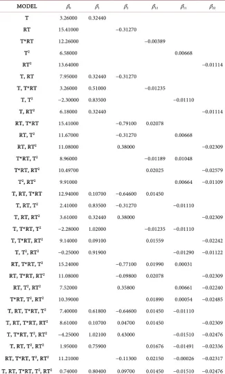
1) Adhesion Response Models

Table A1 shows the summary information of the thirty one all possible gression models generated by Minitab 17 for the adhesion response. Each re-sponse model is shown with its regressors and parameter values. For example, the first and second models which are represented by T and RT expand to:

Adhesion 3.26 0.3244 T= + ∗ ₍₅₎

and

Adhesion 15.41 0.3127 RT= − ∗ ₍₆₎

The rest of the twenty nine models are expanded in a similar manner.

DOI: 10.4236/ojs.2019.91010 130 Open Journal of Statistics Table A1. Summary of adhesion models.

MODEL β0 β1 β2 β12 β11 β22

T 3.26000 0.32440

RT 15.41000 −0.31270

T*RT 12.26000 −0.00389

T2 _{6.58000 0.00668}

RT2 _{13.64000 −0.01114}

T, RT 7.95000 0.32440 −0.31270

T, T*RT 3.26000 0.51000 −0.01235

T, T2 _{−2.30000 0.83500 −0.01110}

T, RT2 _{6.18000 0.32440 −0.01114}

RT, T*RT 15.41000 −0.79100 0.02078

RT, T2 _{11.67000 −0.31270 0.00668}

RT, RT2 _{11.08000 0.38000 −0.02309}

T*RT, T2 _{8.96000 −0.01189 0.01048}

T*RT, RT2 _{10.49700 0.02025 −0.02579}

T2_{, RT}2 _{9.91000 0.00664 −0.01109}

T, RT, T*RT 12.94000 0.10700 −0.64600 0.01450

T, RT, T2 _{2.41000 0.83500 −0.31270 −0.01110}

T, RT, RT2 _{3.61000 0.32440 0.38000 −0.02309}

T, T*RT, T2 _{−2.28000 1.02000 −0.01235 −0.01110}

T, T*RT, RT2 _{9.14000 0.09100 0.01559 −0.02242}

T, T2_{, RT}2 _{−0.25000 0.91900 −0.01290 −0.01122}

RT, T*RT, T2 _{15.24000 −0.77100 0.01990 0.00031}

RT, T*RT, RT2 _{11.08000 −0.09800 0.02078 −0.02309}

RT, T2_{, RT}2 _{7.52000 0.35800 0.00661 −0.02240}

T*RT, T2_{, RT}2 _{10.39000 0.01890 0.00054 −0.02485}

T, RT, T*RT, T2 _{7.40000 0.61800 −0.64600 0.01450 −0.01110}

T, RT, T*RT, RT2 _{8.61000 0.10700 0.04700 0.01450 −0.02309}

T, T*RT, T2_{, RT}2 _{−4.25000 1.02100 0.43000 −0.01510 −0.02476}

T, RT, T2_{, RT}2 _{1.95000 0.75900 0.01676 −0.01491 −0.02336}

RT, T*RT, T2_{, RT}2 _{11.21000 −0.11300 0.02150 −0.00026 −0.02317}

T, RT, T*RT, T2_{, RT}2 _{0.74000 0.80400 0.09700 0.01450 −0.01510 −0.02476}

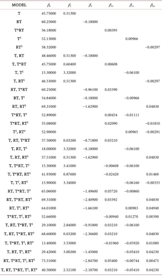
2) Hardness Response Models

DOI: 10.4236/ojs.2019.91010 131 Open Journal of Statistics Table A2. Summary of hardness models.

MODEL β0 β1 β2 β12 β11 β22

T 45.75000 0.51300

RT 60.25000 −0.18000

T*RT 56.18000 0.00395

T2 _{52.13000 0.00966}

RT2 _{58.32000 −0.00297}

T, RT 48.46000 0.51300 −0.18000

T, T*RT 45.75000 0.60400 0.00608

T, T2 _{15.30000 3.32000 −0.06100}

T, RT2 _{46.53000 0.51300 −0.00297}

RT, T*RT 60.25000 −0.96100 0.03390

RT, T2 _{54.84000 −0.18000 −0.00966}

RT, RT2 _{69.31000 −1.62900 0.04830}

T*RT, T2 _{52.89000 0.00454 −0.01111}

T*RT, RT2 _{55.08000 0.02090 −0.01810}

T2_{, RT}2 _{52.90000 0.00965 −0.00291}

T, RT, T*RT 57.50000 0.03200 −0.71800 0.03210

T, RT, T2 _{18.00000 3.32000 −0.18000 −0.06100}

T, RT, RT2 _{57.51000 0.51300 −1.62900 0.04830}

T, T*RT, T2 _{15.30000 3.41000 −0.00608 −0.06100}

T, T*RT, RT2 _{41.93000 0.87600 −0.02420 0.01460}

T, T2_{, RT}2 _{15.90000 3.34000 −0.06160 −0.00335}

RT, T*RT, T2 _{65.06000 −1.49600 0.05720 −0.00860}

RT, T*RT, RT2 _{69.31000 −2.40900 0.03392 0.04830}

RT, T2_{, RT}2 _{64.01000 −1.66100 0.00983 0.04940}

T*RT, T2_{, RT}2 _{52.66000 −0.00940 0.01270 0.00390}

T, RT, T*RT, T2 _{29.10000 2.84000 −0.91800 0.03210 −0.06100}

T, RT, T*RT, RT2 _{68.60000 0.03200 −2.36600 0.03210 0.04830}

T, T*RT, T2_{, RT}2 _{13.40000 3.53000 −0.01960 −0.05920 0.01080}

T, RT, T2_{, RT}2 _{29.42000 3.00200 −1.45000 −0.05410 0.04230}

RT, T*RT, T2_{, RT}2 _{73.31000 −2.84700 0.05400 −0.00744 0.00475}

T, RT, T*RT, T2_{, RT}2 _{40.50000 2.52100 −2.18700 0.03210 −0.05410 0.04230}

Adhesion 45.75 0.513 T= + ∗ (7)

and

Adhesion 60.25 0.18 RT= − ∗ ₍₈₎

DOI: 10.4236/ojs.2019.91010 132 Open Journal of Statistics

Annexure B

1 R² SSR/SST _{correlation coefficient} Squared multiple Goodness of Fit _samples Large

2 R² (adj.) _{1 1− −}

(

)

+ Parsimony samples Large 3 RMSE

(

(

)

)

Predicted Actuali i

i − n

∑

4 MS (LOF) (RSS SSpe− ) (n p− −dpe) Mean Square

Lack of Fit Lack of Fit sample size Any 5 PRESS

∑

(

)

Prediction Sum

of Squares Prediction sample size Any 6 R²-prediction 1 PRESS SSE−( TOT)∗100 Allen (1971b) Prediction _{sample size} Any

7 _Precision Adequate _max

( )

( )

( )

8 Cp

(

)

SSE σ − +n 2p Mallow’s Cp (1973) Prediction _{sample size} Large

9 Cp -p

(

)

SSE σ − +n p _{Mallow’s Cp (1973) Prediction} Large

sample size 10 AIC n∗ln SSE( n)+2k Akaike (1973) Goodness of Fit _{+ Parsimony sample size} Large

11 SBC n∗ln SSE( n k)+ ∗ln( )n Schwarz’s Bayesian

Criterion (1978) Goodness of Fit + Parsimony sample size Large

12 BIC _{n∗ln SSE}( _n)_+2(_k+2)_nσ2 _SSE−₂

( )

    Sawa (1978) Goodness of Fit _{+ Parsimony sample size} Small

13 APCp (n p+ )SSE

(

)

14 AICc AIC 2+ k k( +1) (n k− −1) Corrected AIC,

ugiura (1978) Goodness of Fit + Parsimony sample size Small

15 HQ n∗ln SSE( n)+2p∗ln ln

(

)

Quinn (1979) Goodness of Fit + Parsimony sample size Any 16 HQc ( )2

(

)

ln SSE 2 ln ln 1

n∗ n + np∗ n n p− − Mcquarrie and

Tsai (1998) Goodness of Fit + Parsimony sample size Small

17 KIC n∗ln SSE( n) (+3 k+1) Cavanaugh

J. E. (1999) Goodness of Fit + Parsimony sample size Large 18 KICc n∗ln SSE( n) (+ k+1 3)( n k− −2) (n k− −2)+k n k( − ) _{Bekara M (2004)} Goodness of Fit

+ Parsimony sample sizes Small 19 MKIC _2(_{n P− −2})_σ2_{p σ}2_{p+2p−2n+4}

  Cavanaugh _{J. E. (2004)} Goodness of Fit _{+ Parsimony sample sizes} Small

20 MAIC _{AICc+2p n p}( ₋ )_σ2_{x n p}( ₋ )_σ2_{− −1 2 }(_{n p−} )_σ2_{x n p}( ₋ )_σ2_−12

    Fujikoshi and _{Satoh (1997)} Goodness of Fit _{+ Parsimony sample sizes} Small

21 TIC n∗ln SSE( n) (+2 k+1) Takeuchi Information

Criterion () Goodness of Fit + Parsimony sample size Large 22 Sp RMSp (n p− −1) Hocking ₍₁₉₇₆₎ Prediction _{sample size} Large

DOI: 10.4236/ojs.2019.91010 133 Open Journal of Statistics Continued

24 Pp SSEn _{correlated to R²} Highly Goodness of Fit _{sample size} Large 25 KICchm KIC 2+ (p+1)(p+2) (n p− −2) Hafidi and

Mkhadri (2007) Goodness of Fit + Parsimony sample size Small 26 KICcsb KICchm+p n p( − ) Seghouane A. K.

and Bakara (2004) Goodness of Fit + Parsimony sample size Small 27 KICcc KICcsb+ ∗n ln

(

)

J. E. (2004) Goodness of Fit + Parsimony sample size Small 28 mMDL ( )n2 ln RSS

(

)

and Bin Yu (2001) Goodness of Fit + Parsimony sample size Any 29 gMDL ( )n2 ln RSS

(

)

and Bin Yu (2001) Goodness of Fit + Parsimony sample size Any

Annexure C

The four adhesion and one hardness conforming response surfaces constructed using excel are shown.

1) Adhesion [T, RT, T*RT] (Figure C1)

Figure C1. Showing the adhesion response surface for the model.

2) Adhesion [T, RT, T*RT, T2_{] Response Surface (Figure C2)}

Figure C2. Showing the adhesion response surface for the model [T, RT, T*RT, T2_].

DOI: 10.4236/ojs.2019.91010 134 Open Journal of Statistics Figure C3. Showing the response surface of the adhesion model [T, RT, T*RT, RT2_].

4) Adhesion [T, RT, T*RT, T2_{, RT}2_{] Response Surface (Figure C4)}

Figure C4. Showing the conforming response surface for the adhesion model [T, RT, T*RT, T2_{, RT}2_].

The four adhesion response surfaces show the expected continuously rising modulus behaviour of rubber skim compounds whose specification is synthetic rubber based.

5) Hardness [T, RT, T*RT, T2_]

The response surface for [T, RT, T*RT, T2_{] is the only conforming response}

surface for hardness among the thirty one hardness models and is shown in

Figure C5.

Figure C5. Showing the hardness response surface from the single conforming response surface model.

DOI: 10.4236/ojs.2019.91010 135 Open Journal of Statistics

Annexure D

1) Response surfaces, data matrices and determination of results a) Data Matrices

i) Adhesion [T, RT, T*RT] (Table D1)

Table D1. Showing the data matrix of the adhesion model [T, RT, T*RT].

CT

RT 21 22 23 24 25 26 27 28 29 30 20 8 9 9 10 10 10 11 11 12 12 19 9 9 9 10 10 11 11 11 12 12 18 9 9 10 10 11 11 11 12 12 12 17 9 10 10 10 11 11 11 12 12 13 16 10 10 10 11 11 11 12 12 12 13 15 10 10 11 11 11 12 12 12 13 13 14 10 11 11 11 12 12 12 13 13 13 13 11 11 11 12 12 12 13 13 13 13 12 11 11 12 12 12 13 13 13 13 14 11 11 12 12 12 13 13 13 13 14 14 10 12 12 12 13 13 13 13 14 14 14 9 12 12 13 13 13 13 14 14 14 14 8 12 13 13 13 13 14 14 14 14 14 7 13 13 13 13 14 14 14 14 14 15

The data matrix for the adhesion model [T, RT, T*RT] if overlapped with a hardness model data matrix from a conforming response surface will give a wanted region with optimum cure time per rubber thickness results.

ii) Hardness [T, RT, T*RT, T2_{] (Table D2)}

Table D2. Showing the data matrix of the hardness model [T, RT, T*RT, T2_].

CT

DOI: 10.4236/ojs.2019.91010 136 Open Journal of Statistics

The hardness data matrix for model [T, RT, T*RT, T2_{] will overlap with any}

conforming response model to give the optimum region with cure time per rub-ber thickness results.

Table D3 shows the region in red in which both the adhesion and hardness are within the customer specified region of adhesion ≥ 12 N/mm and hardness ≥ 60 Shore A.

Table D3. Showing the customer specified region in red.

CT

RT 21 22 23 24 25 26 27 28 29 30

20 60 60

19 60 60

18 61 60 60

17 61 60 60

16 61 61 60 60

15 61 61 61 60 60

14 60 61 61 61 60 60

13 60 61 61 61 61 60 60

12 60 60 61 61 61 61 60 60

11 60 60 61 61 61 61 61 60 60

10 60 60 60 61 61 61 61 61 60 60

9 60 60 61 61 61 61 61 61 60 60

8 60 60 61 61 61 61 61 61 60 60

7 60 61 61 61 61 61 61 61 60 60

2) Pair 2: [T, RT, T*RT, T2_{] vs. [T, RT, T*RT, T}2_]

a) Response Surfaces

i) Adhesion [T, RT, T*RT, T2_{] (Figure D1)}

Figure D1. Showing the adhesion response surface for the model [T, RT, T*RT, T2_].

DOI: 10.4236/ojs.2019.91010 137 Open Journal of Statistics Figure D2. Showing the hardness response surface for [T, RT, T*RT, T2_].

b) Data Matrices

i) Adhesion [T, RT, T*RT, T2_{] (Table D4)}

Table D4. Summarising model selection results split between fit to data, prediction and conforming response surface.

CT

RT 21 22 23 24 25 26 27 28 29 30 20 9 9 9 10 10 11 11 11 11 12 19 9 9 10 10 11 11 11 11 12 12 18 9 10 10 10 11 11 11 12 12 12 17 10 10 10 11 11 11 12 12 12 12 16 10 10 11 11 11 12 12 12 12 13 15 10 11 11 11 12 12 12 12 13 13 14 11 11 11 12 12 12 12 13 13 13 13 11 11 12 12 12 12 13 13 13 13 12 11 12 12 12 13 13 13 13 13 13 11 12 12 12 13 13 13 13 13 14 14 10 12 12 13 13 13 13 13 14 14 14 9 12 13 13 13 13 14 14 14 14 14 8 13 13 13 13 14 14 14 14 14 14 7 13 13 14 14 14 14 14 14 14 14

ii) Hardness [T, RT, T*RT, T2_{] (Table D5 and Table D6)}

Table D5. Showing the data matrix of the hardness model [T, RT, T*RT, T2_].

CT

DOI: 10.4236/ojs.2019.91010 138 Open Journal of Statistics Continued

15 58 59 60 60 60 61 61 61 60 60 14 59 59 60 60 60 61 61 61 60 60 13 59 59 60 60 61 61 61 61 60 60 12 59 60 60 60 61 61 61 61 60 60 11 59 60 60 61 61 61 61 61 60 60 10 60 60 60 61 61 61 61 61 60 60 9 60 60 61 61 61 61 61 61 60 60 8 60 60 61 61 61 61 61 61 60 60 7 60 61 61 61 61 61 61 61 60 60

Table D6. Showing the customer specified region of Pair 2 in red.

CT

RT 21 22 23 24 25 26 27 28 29 30

20 60

19 60 60

18 61 60 60

17 61 61 60 60

16 60 61 61 60 60

15 60 61 61 61 60 60

14 60 60 61 61 61 60 60

13 60 60 61 61 61 61 60 60

12 60 60 60 61 61 61 61 60 60

11 60 60 61 61 61 61 61 60 60

10 60 60 60 61 61 61 61 61 60 60

9 60 60 61 61 61 61 61 61 60 60

8 60 60 61 61 61 61 61 61 60 60

7 60 61 61 61 61 61 61 61 60 60

3) Pair 3: [T, RT, T*RT, RT2_{] vs. [T, RT, T*RT, T}2_]

a) Response Surfaces

i) Adhesion [T, RT, T*RT, RT2_{] (Figure D3)}

DOI: 10.4236/ojs.2019.91010 139 Open Journal of Statistics

ii) Hardness [T, RT, T*RT, T2_]

The hardness response surface is shown already in Figure D2 above. b) Data Matrices

i) Adhesion [T, RT, T*RT, RT2_{] (Table D7)}

Table D7. Summarising model selection results split between fit to data, prediction and conforming response surface.

CT

RT 21 22 23 24 25 26 27 28 29 30 20 9 9 9 10 10 11 11 11 11 12 19 9 9 10 10 11 11 11 11 12 12 18 9 10 10 10 11 11 11 12 12 12 17 10 10 10 11 11 11 12 12 12 12 16 10 10 11 11 11 12 12 12 12 13 15 10 11 11 11 12 12 12 12 13 13 14 11 11 11 12 12 12 12 13 13 13 13 11 11 12 12 12 12 13 13 13 13 12 11 12 12 12 13 13 13 13 13 13 11 12 12 12 13 13 13 13 13 14 14 10 12 12 13 13 13 13 13 14 14 14 9 12 13 13 13 13 14 14 14 14 14 8 13 13 13 13 14 14 14 14 14 14 7 13 13 14 14 14 14 14 14 14 14

ii) Hardness [T, RT, T*RT, T2_{] (Table D8 and Table D9)}

Table D8. Showing the data matrix of the hardness model [T, RT, T*RT, T2_].

CT

DOI: 10.4236/ojs.2019.91010 140 Open Journal of Statistics Table D9. Showing the customer specified region of Pair 3 in red.

CT

RT 21 22 23 24 25 26 27 28 29 30

20 60

19 60 60

18 61 60 60

17 61 61 60 60

16 60 61 61 60 60

15 60 61 61 61 60 60

14 60 60 61 61 61 60 60

13 60 60 61 61 61 61 60 60

12 60 60 60 61 61 61 61 60 60

11 60 60 61 61 61 61 61 60 60

10 60 60 60 61 61 61 61 61 60 60

9 60 60 61 61 61 61 61 61 60 60

8 60 60 61 61 61 61 61 61 60 60

7 60 61 61 61 61 61 61 61 60 60

4) Pair 4: [T, RT, T*RT, T2_{, RT}2_{] vs. [T, RT, T*RT, T}2_]

a) Response Surfaces

i) Adhesion [T, RT, T*RT, T2_{, RT}2_{] (Figure D4)}

Figure D4. Showing the response surface of the adhesion model [T, RT, T*RT, T2_{, RT}2_].

ii) Hardness [T, RT, T*RT, T2_]

The hardness response surface is shown in D2 above. b) Data Matrices

DOI: 10.4236/ojs.2019.91010 141 Open Journal of Statistics Table D10. Showing the data matrix of the adhesion model [T, RT, T*RT, T2_{, RT}2_].

CT

RT 21 22 23 24 25 26 27 28 29 30 20 9 10 10 10 11 11 11 12 12 12 19 10 10 10 11 11 11 12 12 12 12 18 10 11 11 11 12 12 12 12 13 13 17 11 11 11 12 12 12 13 13 13 13 16 11 11 12 12 12 13 13 13 13 13 15 11 12 12 12 13 13 13 13 14 14 14 12 12 12 13 13 13 13 14 14 14 13 12 12 13 13 13 13 14 14 14 14 12 12 13 13 13 13 14 14 14 14 14 11 12 13 13 13 13 14 14 14 14 14 10 12 13 13 13 13 14 14 14 14 14 9 13 13 13 13 14 14 14 14 14 14 8 13 13 13 13 13 14 14 14 14 14 7 13 13 13 13 13 14 14 14 14 14

Table D11. Showing the data matrix of the hardness model [T, RT, T*RT, T2_].

CT

DOI: 10.4236/ojs.2019.91010 142 Open Journal of Statistics Table D12. Showing the customer specified region of Pair 4 in red.

CT

RT 21 22 23 24 25 26 27 28 29 30

20 60 60 60

19 60 61 60 60

18 60 60 60 61 60 60

17 60 60 60 61 61 60 60

16 60 60 60 61 61 60 60

15 60 60 60 61 61 61 60 60

14 60 60 60 61 61 61 60 60

13 60 60 61 61 61 61 60 60

12 60 60 60 61 61 61 61 60 60

11 60 60 61 61 61 61 61 60 60

10 60 60 60 61 61 61 61 61 60 60

9 60 60 61 61 61 61 61 61 60 60

8 60 60 61 61 61 61 61 61 60 60

7 60 61 61 61 61 61 61 61 60 60

2) Results See Table D13.

Table D13. Showing rubber thickness—Cure Time optimum combinations for the four pairs of adhesion vs. hardness models. (a) Pair 1: [T, RT, T*RT] vs. [T, RT, T*RT, T2_{]; (b)} Pair 2: [T, RT, T*RT, T2_{] vs. [T, RT, T*RT, T}2_{]; (c) Pair 3: [T, RT, T*RT, RT}2_{] vs. [T, RT,} T*RT, T2_{]; (d) Pair 4: [T, RT, T*RT, T}2_{, RT}2_{] vs. [T, RT, T*RT, T}2_].

(a)

Rubber Thickness (mm) 7 8 9 10 11 12 13 14 15 16 17 18 19 20 Cure Time (min.) 21 22 23 24 24 25 25 26 26 27 28 28 29 30

(b)

Rubber Thickness (mm) 7 8 9 10 11 12 13 14 15 16 17 18 19 20 Cure Time (min.) 21 22 23 24 24 25 25 26 26 27 27 28 29 30

(c)

Rubber Thickness (mm) 7 8 9 10 11 12 13 14 15 16 17 18 19 20 Cure Time (min.) 21 22 23 24 24 25 25 26 26 27 27 28 29 30

(d)